[R-bloggers] Forget about Excel, Use these R Shiny Packages Instead (and 2 more aRticles)

---

• Forget about Excel, Use these R Shiny Packages Instead
• Analyzing a binary outcome arising out of within-cluster, pair-matched randomization
• Spatial regression in R part 1: spaMM vs glmmTMB

Forget about Excel, Use these R Shiny Packages Instead Posted: 03 Sep 2019 12:58 AM PDT [This article was first published on r – Appsilon Data Science | End­ to­ End Data Science Solutions, and kindly contributed to R-bloggers]. (You can report issue about the content on this page here) Want to share your content on R-bloggers? click here if you have a blog, or here if you don't. tl; dr Transferring your Excel sheet to a Shiny app can be the easiest way to create an enterprise ready dashboard. In this post, I  present 6 Shiny alternatives for the table-like data that Excel users love. Intro  Excel has its limitations regarding advanced statistics and calculations, quality and version control, user experience and scalability. Switching to a more sophisticated data analysis tool or a dashboard is often an answer. Transferring your Excel sheet to a Shiny app can be the easiest way to create an enterprise ready dashboard. Take a look at Filip Stachura's article "Excel Is Obsolete" which addresses, from the architecture point of view, when to stick with Excel and when it is time for a change  In this blogpost we'll focus on the functionalities that may be implemented in a Shiny app. You're probably aware of Shiny's cool interactive plot and charts features that are well ahead of what you can do in Excel. What may still prevent you from switching from Excel to a more advanced Shiny dashboard is the fear of missing the beloved Excel functionalities to work with table-like data. Don't worry! It is super easy to implement and extend them using Shiny. The most commonly used table widgets in Shiny are DT and rhandsontable. Let's take a deep dive into their features but also look at some other packages strictly dedicated to help with popular spreadsheets tasks.   1. Editable tables A basic reason for using a spreadsheet is the simplicity of data manipulation. Displaying data is not always enough. Content may require spell checking, fixing, adding rows or columns. The closest solution to what can be found in spreadsheets is rhandsontable. It contains all of the cool spreadsheet features like autocomplete, selecting a value from a list, adding row/column, sparklines in cells, freezing, comments, input validation, read only mode, and so on. Source: http://jrowen.github.io/rhandsontable/ A similar solution is available in excelR. The package is worth testing as it contains many interesting solutions such as radio selection inside table and the multiple well-known Excel functions, like SUM presented below. The package also allows users to easily manipulate cells with actions like resizing, merging or switching row/column positions. Nested headers are also useful as they can organize your data. Implementing the solution in Shiny is easy and intuitive with well-known render/output dedicated functions. There are two downsides with excelR at the moment — cloning formulas between columns, and calculation approximations, which do not work as one would expect. Source: https://swechhya.github.io/excelR The DT package has a lot of great features and is a great option when heavy data editing is not the main goal. And as you can see in the gif below, tables implemented with DT look really nice. It has less functionality than rhandsontable though, basically just allowing the user to replace the values inside cells when double-clicked, without validating the values typed in. Some columns may be restricted to be read-only. Source: https://rstudio.github.io/DT/ A possible workaround for DT's limited editing functionality is a more advanced DTedit package. It comes with a pleasing interface (modal dialog) for editing single table rows as well as buttons to add, delete or copy data. The package is currently only available on GitHub, but we will keep our fingers crossed for its expansion and increase in popularity. Source: https://github.com/jbryer/DTedit 2. Conditional formatting Conditional formatting is a super useful tool for getting a quick overview when dealing with tons of values. Both rhandsontable and DT allow users to format cells according to its values. If your highest priority for your application is beautiful data presentation, then the package formattable is worth checking out. The formatting interface is more user-friendly than in rhandsontable and it is based on R functions, not pure javascript code. Besides working on tables, it also contains functionality of formatting R vectors which might be useful when presenting results of pure R analysis. Source: https://github.com/renkun-ken/formattable   3. Sorting and filtering Sorting and filtering are also crucial when examining a huge dataset. In the rhandsontable package, sorting columns can be enabled by a single parameter, however filtering is not implemented inside the feature and may require adding some extra Shiny components. On the other hand, in DT, column sorting is available by default as well as global search. Enabling column filtering is as easy as adding a single parameter (filter = top/bottom, depending on where the filters should be placed).  Source: https://rstudio.github.io/DT/ 4. Drag & drop pivot tables Excel users love pivot tables. Allowing the users to create their own stories based on data is an excellent feature – sometimes the valuable info is only generated when looking at the data from the right angle. For a plug-and-play pivot table we recommend using the rpivotTable package. As you can see in the gif, it is super easy to produce tables and manipulate the aggregation variables with drag & drop. You can also filter by specific values and/or choose which variable should be calculated based on the selected function – like presented below sum and sum as percentage of total. Quickly switching from table to different types of (interactive!) charts is a great bonus. Source: https://github.com/smartinsightsfromdata/rpivotTable If you would like to combine pivoting with other features, a combination of shinydnd and DT Custom Table Containers as well as data manipulation is needed. Nevertheless, the results can be amazing. Maybe we'll get into that in a future post.   5. Reacting on selection The usual scenario in dashboards applications is reacting to user selection and continuing to work on a selected element. When it needs to be a key feature of the application, then the DT package is a great choice. It is easy to implement logic for reacting to user cell/row/column selection.    The sky's the limit really! Options range from custom edit data tools to going deep into nested tables. Or as presented in the gif below, you see the graph dynamically reacts to user selection in the table. Source: https://rstudio.github.io/DT/shiny.html 6. Expandable rows …is an extra nice feature that allows you to hide (in an elegant way) additional information and bring the crucial part to the top. This is another feature that does not exist in spreadsheets. Expandable rows is also useful in presenting database-like structures with one-to-many relations. It requires a little javascript magic in DT for now, but the various examples (including this one) are easy to follow. Source: http://www.reigo.eu/2018/04/extending-dt-child-row-example/ Conclusion You may have felt that if you switched from Excel to Shiny, you would be limited in the table data feature set. I hope you can see by now that Shiny offers a comparable feature set to Excel as well as exciting new possibilities! You can reach me on Twitter @DubelMarcin. Article Forget about Excel, Use these R Shiny Packages Instead comes from Appsilon Data Science | End­ to­ End Data Science Solutions. To leave a comment for the author, please follow the link and comment on their blog: r – Appsilon Data Science | End­ to­ End Data Science Solutions. R-bloggers.com offers daily e-mail updates about R news and tutorials about learning R and many other topics. Click here if you're looking to post or find an R/data-science job. Want to share your content on R-bloggers? click here if you have a blog, or here if you don't. This posting includes an audio/video/photo media file: Download Now

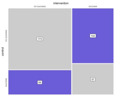
Analyzing a binary outcome arising out of within-cluster, pair-matched randomization Posted: 02 Sep 2019 05:00 PM PDT [This article was first published on ouR data generation, and kindly contributed to R-bloggers]. (You can report issue about the content on this page here) Want to share your content on R-bloggers? click here if you have a blog, or here if you don't. A key motivating factor for the simstudy package and much of this blog is that simulation can be super helpful in understanding how best to approach an unusual, or least unfamiliar, analytic problem. About six months ago, I described the DREAM Initiative (Diabetes Research, Education, and Action for Minorities), a study that used a slightly innovative randomization scheme to ensure that two comparison groups were evenly balanced across important covariates. At the time, we hadn't finalized the analytic plan. But, now that we have started actually randomizing and recruiting (yes, in that order, oddly enough), it is important that we do that, with the help of a little simulation. The study design The original post has the details about the design and matching algorithm (and code). The randomization is taking place at 20 primary care clinics, and patients within these clinics are matched based on important characteristics before randomization occurs. There is little or no risk that patients in the control arm will be "contaminated" or affected by the intervention that is taking place, which will minimize the effects of clustering. However, we may not want to ignore the clustering altogether. Possible analytic solutions Given that the primary outcome is binary, one reasonable procedure to assess whether or not the intervention is effective is McNemar's test, which is typically used for paired dichotomous data. However, this approach has two limitations. First, McNemar's test does not take into account the clustered nature of the data. Second, the test is just that, a test; it does not provide an estimate of effect size (and the associated confidence interval). So, in addition to McNemar's test, I considered four additional analytic approaches to assess the effect of the intervention: (1) Durkalski's extension of McNemar's test to account for clustering, (2) conditional logistic regression, which takes into account stratification and matching, (3) standard logistic regression with specific adjustment for the three matching variables, and (4) mixed effects logistic regression with matching covariate adjustment and a clinic-level random intercept. (In the mixed effects model, I assume the treatment effect does not vary by site, since I have also assumed that the intervention is delivered in a consistent manner across the sites. These may or may not be reasonable assumptions.) While I was interested to see how the two tests (McNemar and the extension) performed, my primary goal was to see if any of the regression models was superior. In order to do this, I wanted to compare the methods in a scenario without any intervention effect, and in another scenario where there was an effect. I was interested in comparing bias, error rates, and variance estimates. Data generation The data generation process parallels the earlier post. The treatment assignment is made in the context of the matching process, which I am not showing this time around. Note that in this initial example, the outcome y depends on the intervention rx (i.e. there is an intervention effect). library(simstudy) ### defining the data defc <- defData(varname = "ceffect", formula = 0, variance = 0.4, dist = "normal", id = "cid") defi <- defDataAdd(varname = "male", formula = .4, dist = "binary") defi <- defDataAdd(defi, varname = "age", formula = 0, variance = 40) defi <- defDataAdd(defi, varname = "bmi", formula = 0, variance = 5) defr <- defDataAdd(varname = "y", formula = "-1 + 0.08*bmi - 0.3*male - 0.08*age + 0.45*rx + ceffect", dist = "binary", link = "logit") ### generating the data set.seed(547317) dc <- genData(20, defc) di <- genCluster(dc, "cid", 60, "id") di <- addColumns(defi, di) ### matching and randomization within cluster (cid) library(parallel) library(Matching) RNGkind("L'Ecuyer-CMRG") # to set seed for parallel process dd <- rbindlist(mclapply(1:nrow(dc), function(x) dmatch(di[cid == x]), mc.set.seed = TRUE ) ) ### generate outcome dd <- addColumns(defr, dd) setkey(dd, pair) dd ## cid ceffect id male age bmi rx pair y ## 1: 1 1.168 11 1 4.35 0.6886 0 1.01 1 ## 2: 1 1.168 53 1 3.85 0.2215 1 1.01 1 ## 3: 1 1.168 51 0 6.01 -0.9321 0 1.02 0 ## 4: 1 1.168 58 0 7.02 0.1407 1 1.02 1 ## 5: 1 1.168 57 0 9.25 -1.3253 0 1.03 1 ## --- ## 798: 9 -0.413 504 1 -8.72 -0.0767 1 9.17 0 ## 799: 9 -0.413 525 0 1.66 3.5507 0 9.18 0 ## 800: 9 -0.413 491 0 4.31 2.6968 1 9.18 0 ## 801: 9 -0.413 499 0 7.36 0.6064 0 9.19 0 ## 802: 9 -0.413 531 0 8.05 0.8068 1 9.19 0 Based on the outcomes of each individual, each pair can be assigned to a particular category that describes the outcomes. Either both fail, both succeed, or one fails and the other succeeds. These category counts can be represented in a \(2 \times 2\) contingency table. The counts are the number of pairs in each of the four possible pairwise outcomes. For example, there were 173 pairs where the outcome was determined to be unsuccessful for both intervention and control arms. dpair <- dcast(dd, pair ~ rx, value.var = "y") dpair[, control := factor(`0`, levels = c(0,1), labels = c("no success", "success"))] dpair[, rx := factor(`1`, levels = c(0, 1), labels = c("no success", "success"))] dpair[, table(control,rx)] ## rx ## control no success success ## no success 173 102 ## success 69 57 Here is a figure that depicts the \(2 \times 2\) matrix, providing a visualization of how the treatment and control group outcomes compare. (The code is in the addendum in case anyone wants to see the lengths I took to make this simple graphic.) McNemar's test McNemar's test requires the data to be in table format, and the test really only takes into consideration the cells which represent disagreement between treatment arms. In terms of the matrix above, this would be the lower left and upper right quadrants. ddc <- dcast(dd, pair ~ rx, value.var = "y") dmat <- ddc[, .N, keyby = .(`0`,`1`)][, matrix(N, 2, 2, byrow = T)] mcnemar.test(dmat) ## ## McNemar's Chi-squared test with continuity correction ## ## data: dmat ## McNemar's chi-squared = 6, df = 1, p-value = 0.01 Based on the p-value = 0.01, we would reject the null hypothesis that the intervention has no effect. Durkalski extension of McNemar's test Durkalski's test also requires the data to be in tabular form, though there essentially needs to be a table for each cluster. The clust.bin.pair function needs us to separate the table into vectors a, b, c, and d, where each element in each of the vectors is a count for a specific cluster. Vector a is collection of counts for the upper left hand quadrants, b is for the upper right hand quadrants, etc. We have 20 clusters, so each of the four vectors has length 20. Much of the work done in the code below is just getting the data in the right form for the function. library(clust.bin.pair) ddc <- dcast(dd, cid + pair ~ rx, value.var = "y") ddc[, ypair := 2*`0` + 1*`1`] dvec <- ddc[, .N, keyby=.(cid, ypair)] allpossible <- data.table(expand.grid(1:20, 0:3)) setnames(allpossible, c("cid","ypair")) setkey(dvec, cid, ypair) setkey(allpossible, cid, ypair) dvec <- dvec[allpossible] dvec[is.na(N), N := 0] a <- dvec[ypair == 0, N] b <- dvec[ypair == 1, N] c <- dvec[ypair == 2, N] d <- dvec[ypair == 3, N] clust.bin.pair(a, b, c, d, method = "durkalski") ## ## Durkalski's Chi-square test ## ## data: a, b, c, d ## chi-square = 5, df = 1, p-value = 0.03 Again, the p-value, though larger, leads us to reject the null. Conditional logistic regression Conditional logistic regression is conditional on the pair. Since the pair is similar with respect to the matching variables, no further adjustment (beyond specifying the strata) is necessary. library(survival) summary(clogit(y ~ rx + strata(pair), data = dd))$coef["rx",] ## coef exp(coef) se(coef) z Pr(>|z|) ## 0.3909 1.4783 0.1559 2.5076 0.0122   Logistic regression with matching covariates adjustment Using logistic regression should in theory provide a reasonable estimate of the treatment effect, though given that there is clustering, I wouldn't expect the standard error estimates to be correct. Although we are not specifically modeling the matching, by including covariates used in the matching, we are effectively estimating a model that is conditional on the pair. summary(glm(y~rx + age + male + bmi, data = dd, family = "binomial"))$coef["rx",] ## Estimate Std. Error z value Pr(>|z|) ## 0.3679 0.1515 2.4285 0.0152   Generalized mixed effects model with matching covariates adjustment The mixed effects model merely improves on the logistic regression model by ensuring that any clustering effects are reflected in the estimates. library(lme4) summary(glmer(y ~ rx + age + male + bmi + (1|cid), data= dd, family = "binomial"))$coef["rx",] ## Estimate Std. Error z value Pr(>|z|) ## 0.4030 0.1586 2.5409 0.0111   Comparing the analytic approaches To compare the methods, I generated 1000 data sets under each scenario. As I mentioned, I wanted to conduct the comparison under two scenarios. The first when there is no intervention effect, and the second with an effect (I will use the effect size used to generate the first data set. I'll start with no intervention effect. In this case, the outcome definition sets the true parameter of rx to 0. defr <- defDataAdd(varname = "y", formula = "-1 + 0.08*bmi - 0.3*male - 0.08*age + 0*rx + ceffect", dist = "binary", link = "logit") Using the updated definition, I generate 1000 datasets, and for each one, I apply the five analytic approaches. The results from each iteration are stored in a large list. (The code for the iterative process is shown in the addendum below.) As an example, here are the contents from the 711th iteration: res[[711]] ## $clr ## coef exp(coef) se(coef) z Pr(>|z|) ## rx -0.0263 0.974 0.162 -0.162 0.871 ## ## $glm ## Estimate Std. Error z value Pr(>|z|) ## (Intercept) -0.6583 0.1247 -5.279 1.30e-07 ## rx -0.0309 0.1565 -0.198 8.43e-01 ## age -0.0670 0.0149 -4.495 6.96e-06 ## male -0.5131 0.1647 -3.115 1.84e-03 ## bmi 0.1308 0.0411 3.184 1.45e-03 ## ## $glmer ## Estimate Std. Error z value Pr(>|z|) ## (Intercept) -0.7373 0.1888 -3.91 9.42e-05 ## rx -0.0340 0.1617 -0.21 8.33e-01 ## age -0.0721 0.0156 -4.61 4.05e-06 ## male -0.4896 0.1710 -2.86 4.20e-03 ## bmi 0.1366 0.0432 3.16 1.58e-03 ## ## $mcnemar ## ## McNemar's Chi-squared test with continuity correction ## ## data: dmat ## McNemar's chi-squared = 0.007, df = 1, p-value = 0.9 ## ## ## $durk ## ## Durkalski's Chi-square test ## ## data: a, b, c, d ## chi-square = 0.1, df = 1, p-value = 0.7 Summary statistics To compare the five methods, I am first looking at the proportion of iterations where the p-value is less then 0.05, in which case we would reject the the null hypothesis. (In the case where the null is true, the proportion is the Type 1 error rate; when there is truly an effect, then the proportion is the power.) I am less interested in the hypothesis test than the bias and standard errors, but the first two methods only provide a p-value, so that is all we can assess them on. Next, I calculate the bias, which is the average effect estimate minus the true effect. And finally, I evaluate the standard errors by looking at the estimated standard error as well as the observed standard error (which is the standard deviation of the point estimates). pval <- data.frame( mcnm = mean(sapply(res, function(x) x$mcnemar$p.value <= 0.05)), durk = mean(sapply(res, function(x) x$durk$p.value <= 0.05)), clr =mean(sapply(res, function(x) x$clr["rx","Pr(>|z|)"] <= 0.05)), glm = mean(sapply(res, function(x) x$glm["rx","Pr(>|z|)"] <= 0.05)), glmer = mean(sapply(res, function(x) x$glmer["rx","Pr(>|z|)"] <= 0.05)) ) bias <- data.frame( clr = mean(sapply(res, function(x) x$clr["rx", "coef"])), glm = mean(sapply(res, function(x) x$glm["rx", "Estimate"])), glmer = mean(sapply(res, function(x) x$glmer["rx", "Estimate"])) ) se <- data.frame( clr = mean(sapply(res, function(x) x$clr["rx", "se(coef)"])), glm = mean(sapply(res, function(x) x$glm["rx", "Std. Error"])), glmer = mean(sapply(res, function(x) x$glmer["rx", "Std. Error"])) ) obs.se <- data.frame( clr = sd(sapply(res, function(x) x$clr["rx", "coef"])), glm = sd(sapply(res, function(x) x$glm["rx", "Estimate"])), glmer = sd(sapply(res, function(x) x$glmer["rx", "Estimate"])) ) sumstat <- round(plyr::rbind.fill(pval, bias, se, obs.se), 3) rownames(sumstat) <- c("prop.rejected", "bias", "se.est", "se.obs") sumstat ## mcnm durk clr glm glmer ## prop.rejected 0.035 0.048 0.043 0.038 0.044 ## bias NA NA 0.006 0.005 0.005 ## se.est NA NA 0.167 0.161 0.167 ## se.obs NA NA 0.164 0.153 0.164 In this first case, where the true underlying effect size is 0, the Type 1 error rate should be 0.05. The Durkalski test, the conditional logistical regression, and the mixed effects model are below that level but closer than the other two methods. All three models provide unbiased point estimates, but the standard logistic regression (glm) underestimates the standard errors. The results from the conditional logistic regression and the mixed effects model are quite close across the board. Here are the summary statistics for a data set with an intervention effect of 0.45. The results are consistent with the "no effect" simulations, except that the standard linear regression model exhibits some bias. In reality, this is not necessarily bias, but a different estimand. The model that ignores clustering is a marginal model (with respect to the site), whereas the conditional logistic regression and mixed effects models are conditional on the site. (I've described this phenomenon here and here.) We are interested in the conditional effect here, so that argues for the conditional models. The conditional logistic regression and the mixed effects model yielded similar estimates, though the mixed effects model had slightly higher power, which is the reason I opted to use this approach at the end of the day. ## mcnm durk clr glm glmer ## prop.rejected 0.766 0.731 0.784 0.766 0.796 ## bias NA NA 0.000 -0.033 -0.001 ## se.est NA NA 0.164 0.156 0.162 ## se.obs NA NA 0.165 0.152 0.162 In this last case, the true underlying data generating process still includes an intervention effect but no clustering. In this scenario, all of the analytic yield similar estimates. However, since there is no guarantee that clustering is not a factor, the mixed effects model will still be the preferred approach. ## mcnm durk clr glm glmer ## prop.rejected 0.802 0.774 0.825 0.828 0.830 ## bias NA NA -0.003 -0.002 -0.001 ## se.est NA NA 0.159 0.158 0.158 ## se.obs NA NA 0.151 0.150 0.150 The DREAM Initiative is supported by the National Institutes of Health National Institute of Diabetes and Digestive and Kidney Diseases R01DK11048. The views expressed are those of the author and do not necessarily represent the official position of the funding organizations.   Addendum: multiple datasets and model estimates gen <- function(nclust, m) { dc <- genData(nclust, defc) di <- genCluster(dc, "cid", m, "id") di <- addColumns(defi, di) dr <- rbindlist(mclapply(1:nrow(dc), function(x) dmatch(di[cid == x]))) dr <- addColumns(defr, dr) dr[] } iterate <- function(ncluster, m) { dd <- gen(ncluster, m) clrfit <- summary(clogit(y ~ rx + strata(pair), data = dd))$coef glmfit <- summary(glm(y~rx + age + male + bmi, data = dd, family = binomial))$coef mefit <- summary(glmer(y~rx + age + male + bmi + (1|cid), data= dd, family = binomial))$coef ## McNemar ddc <- dcast(dd, pair ~ rx, value.var = "y") dmat <- ddc[, .N, keyby = .(`0`,`1`)][, matrix(N, 2, 2, byrow = T)] mc <- mcnemar.test(dmat) # Clustered McNemar ddc <- dcast(dd, cid + pair ~ rx, value.var = "y") ddc[, ypair := 2*`0` + 1*`1`] dvec <- ddc[, .N, keyby=.(cid, ypair)] allpossible <- data.table(expand.grid(1:20, 0:3)) setnames(allpossible, c("cid","ypair")) setkey(dvec, cid, ypair) setkey(allpossible, cid, ypair) dvec <- dvec[allpossible] dvec[is.na(N), N := 0] a <- dvec[ypair == 0, N] b <- dvec[ypair == 1, N] c <- dvec[ypair == 2, N] d <- dvec[ypair == 3, N] durk <- clust.bin.pair(a, b, c, d, method = "durkalski") list(clr = clrfit, glm = glmfit, glmer = mefit, mcnemar = mc, durk = durk) } res <- mclapply(1:1000, function(x) iterate(20, 60))   Code to generate figure library(ggmosaic) dpair <- dcast(dd, pair ~ rx, value.var = "y") dpair[, control := factor(`0`, levels = c(1,0), labels = c("success", "no success"))] dpair[, rx := factor(`1`, levels = c(0, 1), labels = c("no success", "success"))] p <- ggplot(data = dpair) + geom_mosaic(aes(x = product(control, rx))) pdata <- data.table(ggplot_build(p)$data[[1]]) pdata[, mcnemar := factor(c("diff","same","same", "diff"))] textloc <- pdata[c(1,4), .(x=(xmin + xmax)/2, y=(ymin + ymax)/2)] ggplot(data = pdata) + geom_rect(aes(xmin=xmin, xmax=xmax, ymin=ymin, ymax=ymax, fill = mcnemar)) + geom_label(data = pdata, aes(x = (xmin+xmax)/2, y = (ymin+ymax)/2, label=.wt), size = 3.2) + scale_x_continuous(position = "top", breaks = textloc$x, labels = c("no success", "success"), name = "intervention", expand = c(0,0)) + scale_y_continuous(breaks = textloc$y, labels = c("success", "no success"), name = "control", expand = c(0,0)) + scale_fill_manual(values = c("#6b5dd5", "grey80")) + theme(panel.grid = element_blank(), legend.position = "none", axis.ticks = element_blank(), axis.text.x = element_text(angle = 0, hjust = 0.5), axis.text.y = element_text(angle = 90, hjust = 0.5) ) To leave a comment for the author, please follow the link and comment on their blog: ouR data generation. R-bloggers.com offers daily e-mail updates about R news and tutorials about learning R and many other topics. Click here if you're looking to post or find an R/data-science job. Want to share your content on R-bloggers? click here if you have a blog, or here if you don't. This posting includes an audio/video/photo media file: Download Now

Spatial regression in R part 1: spaMM vs glmmTMB Posted: 02 Sep 2019 08:17 AM PDT [This article was first published on R Programming – DataScience+, and kindly contributed to R-bloggers]. (You can report issue about the content on this page here) Want to share your content on R-bloggers? click here if you have a blog, or here if you don't. Are you interested in guest posting? Publish at DataScience+ via your editor (i.e., RStudio). Category Advanced Modeling Tags Data Visualisation GLMM Logistic Regression R Programming spatial model Many datasets these days are collected at different locations over space which may generate spatial dependence. Spatial dependence (observation close together are more correlated than those further apart) violate the assumption of independence of the residuals in regression models and require the use of a special class of models to draw the valid inference. The first thing to realize is that spatial data come in very different forms: areal data (murder rate per county), point pattern (trees in forest – random sampling locations) or point referenced data (soil carbon content – non random sampling locations), and all of these forms have specific models and R packages such as spatialreg for areal data or spatstat for point pattern. In this blog post I will introduce how to perform, validate and interpret spatial regression models fitted in R on point referenced data using Maximum Likelihood with two different packages: (i) spaMM and (ii) glmmTMB. If you, reader, are aware of other packages out there to fit these models do let me know and I'll be happy to include it in this post. Do I need a spatial model? Before plugging into new model complexity, the first question to ask is: "do my dataset require me to take spatial dependence into account?". The basic steps to answer this question are: fit a non-spatial model (lm, glmer …) test for spatial autocorrelation in the residuals (Moran's I …) 3a. No indication of spatial dependence: fine to continue with your non-spatial model 3b. Indication of spatial dependence: fit a spatial model Let's look at this with a first simulated example. In a research project we are interested in understanding the link between tree height and temperature, to achieve this we recorded both parameters in 100 different forests and we want to use regression models. Step 0: data simulation # load libraries library(tidyverse) library(gridExtra) library(NLMR) library(DHARMa) # simulate a random temperature gradient temp <- nlm_distancegradient(ncol = 100, nrow = 100, origin = c(1,10,1,10), rescale = TRUE) # extract the temperature values at 100 random points dat <- data.frame(x = runif(100,0,100), y = runif(100,0,100)) dat$temperature <- raster::extract(temp, dat) # simulate tree height dat$height <- 20 + 35 * dat$temperature + rnorm(100) # plot spatial pattern in tree height ggplot(dat, aes(x = x, y = y, size = height)) + geom_point() + scale_size_continuous(range = c(1,10)) # clear spatial pattern Step 1: fit a non-spatial model # fit a non-spatial model m_non <- lm(height ~ temperature, dat) Step 2: test for spatial autocorrelation in the residuals # plot residuals dat$resid <- resid(m_non) # dat$resid_std <- rescale(dat$resid, 1, 10) ggplot(dat, aes(x = x, y = y, size = resid)) + geom_point() + scale_size_continuous(range = c(1,10)) Visually checking model residuals show that there seems to be little spatial dependency there. p-values fans can also rely on formal test (like Moran's I): # formal test sims <- simulateResiduals(m_non) testSpatialAutocorrelation(sims, x = dat$x, y = dat$y, plot = FALSE) ## ## DHARMa Moran's I test for spatial autocorrelation ## ## data: sims ## observed = -0.020435, expected = -0.010101, sd = 0.016756, p-value ## = 0.5374 ## alternative hypothesis: Spatial autocorrelation No evidence of spatial Autocorrelation. We can go to Step 3a. Step 3a This little toy example showed that even if there are a spatial pattern in the data this does not mean that spatial regression models should be used. In some cases spatial patterns in the response variable are generated by spatial patterns present in the covariates, such as temperature gradient, elevation … Once we take into account the effect of these covariates spatial patterns in the response variable disappear. So before starting to fit a spatial model, one should check that such complexity is warranted by the data. Fitting a spatial regression model The basic model structure that we will consider in this post is: \[ y_i \sim \mathcal{N}(\mu_i, \sigma) \] i index the different observations, y is the response variable (tree height …), \(\mu\) is the linear predictor and \(\sigma\) is the residual standard deviation. The linear predictor is defined as follow: \[ \mu_i = X_i\beta + u(s_i) \] The first term is just a classical regression in matrix notation (X is the design matrix and \(\beta\) is a vector of regression coefficient), the second term is the spatial term (correlated random term) defined as: \[ u(s_i) \sim \mathcal{MVN}(0, F(\theta_1, …, \theta_n)) \] The spatial term u(s) is basically a multivariate normal distribution with a mean vector of 0 and a covariance matrix given by some function with parameters to be estimated from the data. A classical choice is the Matérn function which has two parameters: \(\nu\) (control rate of decay, smaller value means faster decay) and \(\kappa\) (control smoothness, smaller values means lower smoothness). The input to the Matérn function are the distance between two points and the two parameters (\(\nu\) and \(\kappa\), as output we get the correlation matrix between the locations that will be used to get the spatial effect. This model basically translate the expectation that closer observations should be more correlated, the strength of the spatial signal and its decay will have to be estimated from the data and we will explore here two packages to do so: spaMM and glmmTMB. I will show some code to fit the models, interpret the outputs, derive spatial predictions and check model assumptions for all three methods. The dataset library(geoR) library(viridis) data(ca20) # put this in a data frame dat <- data.frame(x = ca20$coords[,1], y = ca20$coords[,2], calcium = ca20$data, elevation = ca20$covariate[,1], region = factor(ca20$covariate[,2])) # plot the data ggplot(dat, aes(x=x, y = y, color =calcium, shape = region)) + geom_point() + scale_color_viridis(option = "A") # fit a no-spatial model m_lm <- lm(calcium ~ elevation + region, dat) # test for spatial autocorrelation sims <- simulateResiduals(m_lm) testSpatialAutocorrelation(sims, dat$x, dat$y, plot = FALSE) ## ## DHARMa Moran's I test for spatial autocorrelation ## ## data: sims ## observed = 0.0594843, expected = -0.0056497, sd = 0.0069140, ## p-value < 2.2e-16 ## alternative hypothesis: Spatial autocorrelation # need to take into account space spaMM spaMM fits mixed-effect models and allow the inclusion of spatial effect in different forms (Matern, Interpolated Markov Random Fields, CAR / AR1) but also provide interesting other features such as non-gaussian random effects or autocorrelated random coefficient (ie group-specific spatial dependency). spaMM uses a syntax close to the one used in lme4, the main function to fit the model is fitme. We will fit the model structure outlined above to the calcium dataset: library(spaMM) # fit the model m_spamm <- fitme(calcium ~ elevation + region + Matern(1 | x + y), data = dat, family = "gaussian") # this take a bit of time # model summary summary(m_spamm) ## formula: calcium ~ elevation + region + Matern(1 | x + y) ## ML: Estimation of corrPars, lambda and phi by ML. ## Estimation of fixed effects by ML. ## Estimation of lambda and phi by 'outer' ML, maximizing p_v. ## Family: gaussian ( link = identity ) ## ------------ Fixed effects (beta) ------------ ## Estimate Cond. SE t-value ## (Intercept) 34.6296 10.311 3.3585 ## elevation 0.8431 1.860 0.4534 ## region2 8.1300 5.062 1.6060 ## region3 14.5586 4.944 2.9448 ## --------------- Random effects --------------- ## Family: gaussian ( link = identity ) ## --- Correlation parameters: ## 1.nu 1.rho ## 0.43286763 0.01161491 ## --- Variance parameters ('lambda'): ## lambda = var(u) for u ~ Gaussian; ## x + y : 105.3 ## # of obs: 178; # of groups: x + y, 178 ## ------------- Residual variance ------------- ## phi estimate was 0.0030988 ## ------------- Likelihood values ------------- ## logLik ## p_v(h) (marginal L): -628.6316 There are two main output interesting here: first are the fixed effect (beta) which are the estimated regression parameters (slopes). Then the correlation parameter nu and rho which represent the strength and the speed of decay in the spatial effect, which we can turn into the actual spatial correlation effect by plotting the estimated correlation between two locations against their distance: dd <- dist(dat[,c("x","y")]) mm <- MaternCorr(dd, nu = 0.43, rho = 0.01) plot(as.numeric(dd), as.numeric(mm), xlab = "Distance between pairs of location [in m]", ylab = "Estimated correlation") So basically locations more than 200m away have a correlation below 0.1. Now we can check the model using DHARMa: sims <- simulateResiduals(m_spamm)< ## Warning in checkModel(fittedModel): DHARMa: fittedModel not in class of ## supported models. Absolutely no guarantee that this will work! ## Unconditional simulation: plot(sims) Looks relatively ok. Now we can predict the effect of elevation and region while controlling for spatial effects: # the effect of elevation newdat <- expand.grid(x = 5000, y = 5200, elevation = seq(3, 7, length.out = 10), region = factor(1, levels = c(1:3))) newdat$calcium <- as.numeric(predict(m_spamm, newdat, re.form = NA)) # re.form = NA used to remove spatial effects newdat$calcium <- newdat$calcium + mean(c(0,fixef(m_spamm)[3:4])) # to remove region effect # get 95% confidence intervals around predictions newdat <- cbind(newdat, get_intervals(m_spamm, newdata = newdat, intervals = "fixefVar", re.form = NA) + mean(c(0,fixef(m_spamm)[3:4]))) gg1 <- ggplot(dat, aes(x = elevation, y = calcium)) + geom_point() + geom_path(data = newdat) + geom_ribbon(data = newdat, aes(ymin = fixefVar_0.025, ymax = fixefVar_0.975), alpha = 0.2) # now for region effect newdat <- data.frame(x = 5000, y = 5200, elevation = mean(dat$elevation), region = factor(1:3)) # averaging out elevation effect newdat$calcium <- as.numeric(predict(m_spamm, newdat, re.form = NA)) # get 95% CI newdat <- cbind(newdat,get_intervals(m_spamm, newdata = newdat, intervals = "fixefVar", re.form = NA)) gg2 <- ggplot(dat, aes(x = region, y = calcium)) + geom_jitter() + geom_point(data = newdat, color = "red", size = 2) + geom_linerange(data = newdat, aes(ymin = fixefVar_0.025, ymax = fixefVar_0.975), color = "red") # plot together grid.arrange(gg1, gg2, ncol = 2) We can also derive prediction at any spatial location provided that we feed in information on the elevation and the region: library(fields) library(raster) # derive a DEM elev_m <- Tps(dat[,c("x","y")], dat$elevation) ## Warning: ## Grid searches over lambda (nugget and sill variances) with minima at the endpoints: ## (GCV) Generalized Cross-Validation ## minimum at right endpoint lambda = 5.669116e-06 (eff. df= 169.1 ) r <- raster(xmn = 4950, xmx = 5970, ymn = 4800, ymx = 5720, resolution = 10) elev <- interpolate(r, elev_m) # for the region info use the limits given in ca20 pp <- SpatialPolygons(list(Polygons(list(Polygon(ca20$reg1)), ID = "reg1"),Polygons(list(Polygon(ca20$reg2)), ID = "reg2"), Polygons(list(Polygon(ca20$reg3)), ID = "reg3"))) region <- rasterize(pp, r) # predict at any location newdat <- expand.grid(x = seq(4960, 5960, length.out = 50), y = seq(4830, 5710, length.out = 50)) newdat$elevation <- extract(elev, newdat[,1:2]) newdat$region <- factor(extract(region, newdat[,1:2])) # remove NAs newdat <- na.omit(newdat) # predict newdat$calcium <- as.numeric(predict(m_spamm, newdat)) (gg_spamm <- ggplot(newdat,aes(x=x, y=y, fill = calcium)) + geom_raster() + scale_fill_viridis()) That's it for spaMM a great, fast and easy way to fit spatial regressions. glmmTMB glmmTMB fits a broad class of GLMM using Template Model Builder. With this package we can fit different covariance structure including spatial Matern. Let's dive right in. library(glmmTMB) # fitst we need to create a numeric factor recording the coordinates of the sampled locations dat$pos <- numFactor(scale(dat$x), scale(dat$y)) # then create a dummy group factor to be used as a random term dat$ID <- factor(rep(1, nrow(dat))) # fit the model m_tmb <- glmmTMB(calcium ~ elevation + region + mat(pos + 0 | ID), dat) # take some time to fit # model summary of fixed effects summary(m_tmb) ## Family: gaussian ( identity ) ## Formula: calcium ~ elevation + region + mat(pos + 0 | ID) ## Data: dat ## ## AIC BIC logLik deviance df.resid ## 1272.9 1298.4 -628.5 1256.9 170 ## ## Random effects: ## ## Conditional model: ## Groups Name Variance Std.Dev. ## Corr ## ## [ reached getOption("max.print") -- omitted 179 rows ] ## Number of obs: 178, groups: ID, 1 ## ## Dispersion estimate for gaussian family (sigma^2): 0.0277 ## ## Conditional model: ## Estimate Std. Error z value Pr(>|z|) ## (Intercept) 33.9307 10.4800 3.238 0.00121 ** ## elevation 0.9764 1.9097 0.511 0.60917 ## region2 8.5945 5.2265 1.644 0.10010 ## region3 14.4099 5.4326 2.652 0.00799 ** ## --- ## Signif. codes: 0 '***' 0.001 '**' 0.01 '*' 0.05 '.' 0.1 ' ' 1 The output from glmmTMB should be familiar to frequent users of lme4, first we have some general model information (family, link, formula, AIC …), then we have the estimation of the random effect variance (estimated at 105 here very close to the value from spaMM), and the last table under "Conditional model" display the estimates for the fixed effects. These are again pretty close to those estimated by spaMM. Before going any further let's check the model fitness. sims <- simulateResiduals(m_tmb) plot(sims) By running these lines we get a warning that glmmTMB does not implement yet unconditional predictions (without random effect) is not yet possible in glmmTMB so one may expect (and we do see) some upward going slopes on the right graphs. Not much to do at this stage, maybe in the (near) future with update to glmmTMB this could be solved. We can look at the predicted spatial effect: # some R magic to extract and re-order the estimated correlation between pairs of locations fit_cor <- matrix(as.numeric(attr(VarCorr(m_tmb)$cond$ID, "correlation")), nrow = 178, ncol = 178, byrow = FALSE, dimnames = attr(attr(VarCorr(m_tmb)$cond$ID, "correlation"),"dimnames")) ff <- dimnames(fit_cor)[[1]] ff <- gsub("pos","",ff) fit_cor2 <- fit_cor[order(match(ff, dat$pos)), order(match(ff, dat$pos))] # plot plot(as.numeric(dd), fit_cor2[lower.tri(fit_cor2)], xlab = "Distance between pairs of location [m]", ylab = "Estimated correlation") We find here a similar picture to the one from spaMM, but this was quite a bit more work to get it and we don't seem to have direct estimation of the Matern parameters that were readily available in spaMM. We can now look at the effect of elevation and region (since there is no way to marginalize over the random effects in glmmTMB we have to get the CI by hand): # the effect of elevation newdat <- data.frame(elevation = seq(3, 7, length = 10), region = factor(1, levels = 1:3)) # turn this into a model matrix mm <- model.matrix(~ elevation + region, newdat) newdat$calcium <- mm %*% fixef(m_tmb)$cond + mean(c(0, fixef(m_tmb)$cond[3:4])) # predicted values removing region effects pvar <- diag(mm %*% tcrossprod(vcov(m_tmb)$cond, mm)) newdat$lci <- newdat$calcium - 1.96 * sqrt(pvar) newdat$uci <- newdat$calcium + 1.96 * sqrt(pvar) gg1 <- ggplot(dat, aes(x = elevation, y = calcium)) + geom_point() + geom_line(data = newdat) + geom_ribbon(data = newdat, aes(ymin = lci, ymax = uci), alpha = 0.2) # the effect of region newdat <- data.frame(elevation = mean(dat$elevation), region = factor(1:3)) # turn this into a model matrix mm <- model.matrix(~ elevation + region, newdat) newdat$calcium <- mm %*% fixef(m_tmb)$cond # predicted values pvar <- diag(mm %*% tcrossprod(vcov(m_tmb)$cond, mm)) newdat$lci <- newdat$calcium - 1.96 * sqrt(pvar) newdat$uci <- newdat$calcium + 1.96 * sqrt(pvar) gg2 <- ggplot(dat, aes(x = region, y = calcium)) + geom_jitter() + geom_point(data = newdat, color = "red", size = 2) + geom_linerange(data = newdat, aes(ymin = lci, ymax = uci), color = "red") # plot together grid.arrange(gg1, gg2, ncol = 2) Looks very close to the picture we got from spaMM, which is reassuring. It is a bit more laborious to get estimation of Confidence Intervals for glmmTMB as of know but in th enear future new implementation of the predict method with a "re.form=NA" argument would allow easier derivation of the CIs. Now let's see how to derive spatial predictions: # predict at any location newdat <- expand.grid(x = seq(4960, 5960, length.out = 50), y = seq(4830, 5710, length.out = 50)) newdat$ID <- factor(rep(1, nrow(newdat))) newdat$elevation <- extract(elev, newdat[,1:2]) newdat$region <- factor(extract(region, newdat[,1:2])) # remove NAs newdat <- na.omit(newdat) newdat$pos <- numFactor(((newdat$x - mean(dat$x)) / sd(dat$x)), ((newdat$y - mean(dat$y)) / sd(dat$y))) # predict in slices of 100 predictions to speed up computation pp <- rep(NA, 1927) for(i in seq(1, 1927, by = 100)){ if(i == 1901){ pp[1901:1927] <- predict(m_tmb, newdat[1901:1927,], allow.new.levels = TRUE) } else{ pp[i:(i+99)] <- predict(m_tmb, newdat[i:(i+99),], allow.new.levels = TRUE) } # print(i) } newdat$calcium <- pp (gg_tmb <- ggplot(newdat,aes(x=x, y=y, fill = calcium)) + geom_raster() + scale_fill_viridis()) Very similar map to spaMM. Conclusion Time to wrap up what we've seen here. First off, before plunging into spatial regression models you should first check that your covariates do not already take into account the spatial patterns present in your data. Remember that in the implementation of the spatial models discussed here, spatial effects are modelled in a similar fashion to random effects (basically random effect take into account structure in the data be it by design or spatial or temporal structure). So any variation (including spatial) that can be explained by the fixed effects will be taken into account and only remaining variation based on the spatial structure will be effectively going into the estimated spatial effects. Now I presented here two ways to fit similar spatial regression models in R, time to compare a bit their performance and their pros and cons. spaMM is a very nice package, it can handle a relatively large range of response distributions and can fit different form of spatial effects, it implements a synthax close to the classical lme4 one, and in the example tested here it fitted the model relatively fast. It also provides methods to derive predictions and confidence intervals and the general-purpose model checking package DHARMa works with spaMM objects. glmmTMB is a multi-purpose GLMM fitting package with a few extension into structured covariance matrices including spatial effects. The biggest issues with glmmTMB for spatial data are that model fitting is particularly slower than spaMM, deriving unconditional predictions (without spatial effects) is currently not possible and so DHARMa does not work properly and we need to do some stats wizardy to interprete and predict from a fitted model. In a second part we will explore Bayesian ways to do spatial regression in R with the same dataset, stay tuned for more fun! Related Post Find the best predictive model using R/caret package/modelgrid Variable Selection Methods: Lasso and Ridge Regression in Python Bootstrap with Monte Carlo Simulation in Python Monte Carlo Simulation and Statistical Probability Distributions in Python K-Nearest Neighbors (KNN) with Python To leave a comment for the author, please follow the link and comment on their blog: R Programming – DataScience+. R-bloggers.com offers daily e-mail updates about R news and tutorials about learning R and many other topics. Click here if you're looking to post or find an R/data-science job. Want to share your content on R-bloggers? click here if you have a blog, or here if you don't. This posting includes an audio/video/photo media file: Download Now

You are subscribed to email updates from R-bloggers. To stop receiving these emails, you may unsubscribe now.	Email delivery powered by Google
Google, 1600 Amphitheatre Parkway, Mountain View, CA 94043, United States