[R-bloggers] A brief primer on Variational Inference (and 14 more aRticles) |  |
- A brief primer on Variational Inference
- 81st TokyoR Meetup Roundup: A Special Session in {Shiny}!
- The Mysterious Case of the Ghost Interaction
- Non-randomly missing data is hard, or why weights won’t solve your survey problems and you need to think generatively
- Enlarging the eBook supply
- What’s new in DALEX v 0.4.9?
- Extracting basic Plots from Novels: Dracula is a Man in a Hole
- (Re)introducing skimr v2 – A year in the life of an open source R project
- An Amazon SDK for R!?
- Sept 2019: “Top 40” New R Packages
- Mocking is catching
- Any one interested in a function to quickly generate data with many predictors?
- Dogs of New York
- Spelunking macOS ‘ScreenTime’ App Usage with R
- The Chaos Game: an experiment about fractals, recursivity and creative coding
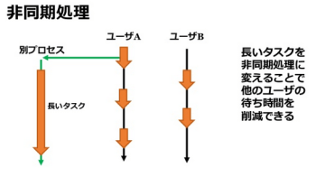
| A brief primer on Variational Inference Posted: 30 Oct 2019 05:00 AM PDT [This article was first published on Fabian Dablander, and kindly contributed to R-bloggers]. (You can report issue about the content on this page here) Want to share your content on R-bloggers? click here if you have a blog, or here if you don't. Bayesian inference using Markov chain Monte Carlo methods can be notoriously slow. In this blog post, we reframe Bayesian inference as an optimization problem using variational inference, markedly speeding up computation. We derive the variational objective function, implement coordinate ascent mean-field variational inference for a simple linear regression example in R, and compare our results to results obtained via variational and exact inference using Stan. Sounds like word salad? Then let's start unpacking! PreliminariesBayes' rule states that where $\mathbf{z}$ denotes latent parameters we want to infer and $\mathbf{x}$ denotes data.1 Bayes' rule is, in general, difficult to apply because it requires dealing with a potentially high-dimensional integral — the marginal likelihood. Optimization, which involves taking derivatives instead of integrating, is much easier and generally faster than the latter, and so our goal will be to reframe this integration problem as one of optimization. Variational objectiveWe want to get at the posterior distribution, but instead of sampling we simply try to find a density $q^\star(\mathbf{z})$ from a family of densities $\mathrm{Q}$ that best approximates the posterior distribution: where $\text{KL}(. \lvert \lvert.)$ denotes the Kullback-Leibler divergence: We cannot compute this Kullback-Leibler divergence because it still depends on the nasty integral $p(\mathbf{x}) = \int p(\mathbf{x} \mid \mathbf{z}) \, p(\mathbf{z}) \, \mathrm{d}\mathbf{z}$. To see this dependency, observe that: where we have expanded the expectation to more clearly behold our nemesis. In doing so, we have seen that $\text{log } p(\mathbf{x})$ is actually a constant with respect to $q(\mathbf{z})$; this means that we can ignore it in our optimization problem. Moreover, minimizing a quantity means maximizing its negative, and so we maximize the following quantity: We can expand the joint probability to get more insight into this equation: This is cool. It says that maximizing the ELBO finds an approximate distribution $q(\mathbf{z})$ for latent quantities $\mathbf{z}$ that allows the data to be predicted well, i.e., leads to a high expected log likelihood, but that a penalty is incurred if $q(\mathbf{z})$ strays far away from the prior $p(\mathbf{z})$. This mirrors the usual balance in Bayesian inference between likelihood and prior (Blei, Kucukelbier, & McAuliffe, 2017). ELBO stands for evidence lower bound. The marginal likelihood is sometimes called evidence, and we see that ELBO is indeed a lower bound for the evidence: since the Kullback-Leibler divergence is non-negative. Heuristically, one might then use the ELBO as a way to select between models. For more on predictive model selection, see this and this blog post. Why variational?Our optimization problem is about finding $q^\star(\mathbf{z})$ that best approximates the posterior distribution. This is in contrast to more familiar optimization problems such as maximum likelihood estimation where one wants to find, for example, the single best value that maximizes the log likelihood. For such a problem, one can use standard calculus (see for example this blog post). In our setting, we do not want to find a single best value but rather a single best function. To do this, we can use variational calculus from which variational inference derives its name (Bishop, 2006, p. 462). A function takes an input value and returns an output value. We can define a functional which takes a whole function and returns an output value. The entropy of a probability distribution is a widely used functional: which takes as input the probability distribution $p(x)$ and returns a single value, its entropy. In variational inference, we want to find the function that minimizes the ELBO, which is a functional. In order to make this optimization problem more manageable, we need to constrain the functions in some way. One could, for example, assume that $q(\mathbf{z})$ is a Gaussian distribution with parameter vector $\omega$. The ELBO then becomes a function of $\omega$, and we employ standard optimization methods to solve this problem. Instead of restricting the parametric form of the variational distribution $q(\mathbf{z})$, in the next section we use an independence assumption to manage the inference problem. Mean-field variational familyA frequently used approximation is to assume that the latent variables $z_j$ for $j = \{1, \ldots, m\}$ are mutually independent, each governed by their own variational density: Note that this mean-field variational family cannot model correlations in the posterior distribution; by construction, the latent parameters are mutually independent. Observe that we do not make any parametric assumption about the individual $q_j(z_j)$. Instead, their parametric form is derived for every particular inference problem. We start from our definition of the ELBO and apply the mean-field assumption: In the following, we optimize the ELBO with respect to a single variational density $q_j(z_j)$ and assume that all others are fixed: One could use variational calculus to derive the optimal variational density $q_j^\star(z_j)$; instead, we follow Bishop (2006, p. 465) and define the distribution where we need to make sure that it integrates to one by subtracting the (log) normalizing constant $\mathcal{Z}$. With this in mind, observe that: Thus, maximizing the ELBO with respect to $q_j(z_j)$ is minimizing the Kullback-leibler divergence between $q_j(z_j)$ and $\tilde{p}(\mathbf{x}, z_j)$; it is zero when the two distributions are equal. Therefore, under the mean-field assumption, the optimal variational density $q_j^\star(z_j)$ is given by: see also Bishop (2006, p. 466). This is not an explicit solution, however, since each optimal variational density depends on all others. This calls for an iterative solution in which we first initialize all factors $q_j(z_i)$ and then cycle through them, updating them conditional on the updates of the other. Such a procedure is known as Coordinate Ascent Variational Inference (CAVI). Further, note that which allows us to write the updates in terms of the conditional posterior distribution of $z_j$ given all other factors $\mathbf{z}_{-j}$. This looks a lot like Gibbs sampling, which we discussed in detail in a previous blog post. In the next section, we implement CAVI for a simple linear regression problem. Application: Linear regressionIn a previous blog post, we traced the history of least squares and applied it to the most basic problem: fitting a straight line to a number of points. Here, we study the same problem but swap optimization procedure: instead of least squares or maximum likelihood, we use variational inference. Our linear regression setup is: where we assume that the population mean of $y$ is zero (i.e., $\beta_0 = 0$); and we assign the error variance $\sigma^2$ an improper Jeffreys' prior and $\beta$ a Gaussian prior with variance $\sigma^2\tau^2$. We scale the prior of $\beta$ by the error variance to reason in terms of a standardized effect size $\beta / \sigma$ since with this specification: As a heads up, we have to do a surprising amount of calculations to implement variational inference even for this simple problem. In the next section, we start our journey by deriving the variational density for $\sigma^2$. Variational density for $\sigma^2$Our optimal variational density $q^\star(\sigma^2)$ is given by: To get started, we need to derive the conditional posterior distribution $p(\sigma^2 \mid \mathbf{y}, \beta)$. We write: which is proportional to an inverse Gamma distribution. Moving on, we exploit the linearity of the expectation and write: This, too, looks like an inverse Gamma distribution! Plugging in the normalizing constant, we arrive at: Note that this quantity depends on $\beta$. In the next section, we derive the variational density for $\beta$. Variational density for $\beta$Our optimal variational density $q^\star(\beta)$ is given by: and so we again have to derive the conditional posterior distribution $p(\beta \mid \mathbf{y}, \sigma^2)$. We write: where we have "completed the square" (see also this blog post) and realized that the conditional posterior is Gaussian. We continue by taking expectations: which is again proportional to a Gaussian distribution! Plugging in the normalizing constant yields: Note that while the variance of this distribution, $\sigma^2_\beta$, depends on $q(\sigma^2)$, its mean $\mu_\beta$ does not. To recap, instead of assuming a parametric form for the variational densities, we have derived the optimal densities under the mean-field assumption, that is, under the assumption that the parameters are independent: $q(\beta, \sigma^2) = q(\beta) \, q(\sigma^2)$. Assigning $\beta$ a Gaussian distribution and $\sigma^2$ a Jeffreys's prior, we have found that the variational density for $\sigma^2$ is an inverse Gamma distribution and that the variational density for $\beta$ a Gaussian distribution. We noted that these variational densities depend on each other. However, this is not the end of the manipulation of symbols; both distributions still feature an expectation we need to remove. In the next section, we expand the remaining expectations. Removing expectationsNow that we know the parametric form of both variational densities, we can expand the terms that involve an expectation. In particular, for the variational density $q^\star(\sigma^2)$ we write: Noting that $\mathbb{E}_{q(\beta)}[\beta] = \mu_{\beta}$ and using the fact that: the expectation becomes: For the expectation which features in the variational distribution for $\beta$, things are slightly less elaborate, although the result also looks unwieldy. Note that since $\sigma^2$ follows an inverse Gamma distribution, $1 / \sigma^2$ follows a Gamma distribution which has mean: Monitoring convergenceThe algorithm works by first specifying initial values for the parameters of the variational densities and then iteratively updating them until the ELBO does not change anymore. This requires us to compute the ELBO, which we still need to derive, on each update. We write: Let's take a deep breath and tackle the second term first: Note that there are three expectations left. However, we really deserve a break, and so instead of analytically deriving the expectations we compute $\mathbb{E}_{q(\sigma^2)}\left[\text{log } \sigma^2\right]$ and $\mathbb{E}_{p(\sigma^2)}\left[\text{log } q(\sigma^2)\right]$ numerically using Gaussian quadrature. This fails for $\mathbb{E}_{q(\sigma^2)}\left[\text{log } q(\sigma^2)\right]$, which we compute using Monte carlo integration:
We are left with the expected log likelihood. Instead of filling this blog post with more equations, we again resort to numerical methods. However, we refactor the expression so that numerical integration is more efficient: Since we have solved a similar problem already above, we evaluate the expecation with respect to $q(\beta)$ analytically:
In the next section, we implement the algorithm for our linear regression problem in R. Implementation in RNow that we have derived the optimal densities, we know how they are parameterized. Therefore, the ELBO is a function of these variational parameters and the parameters of the priors, which in our case is just $\tau^2$. We write a function that computes the ELBO: The function below implements coordinate ascent mean-field variational inference for our simple linear regression problem. Recall that the variational parameters are: The following function implements the iterative updating of these variational parameters until the ELBO has converged. Let's run this on a simulated data set of size $n = 100$ with a true coefficient of $\beta = 0.30$ and a true error variance of $\sigma^2 = 1$. We assign $\beta$ a Gaussian prior with variance $\tau^2 = 0.25$ so that values for $\lvert \beta \rvert$ larger than two standard deviations ($0.50$) receive about $0.68$ prior probability. From the output, we see that the ELBO and the variational parameters have converged. In the next section, we compare these results to results obtained with Stan. Comparison with StanWhenever one goes down a rabbit hole of calculations, it is good to sanity check one's results. Here, we use Stan's variational inference scheme to check whether our results are comparable. It assumes a Gaussian variational density for each parameter after transforming them to the real line and automates inference in a "black-box" way so that no problem-specific calculations are required (see Kucukelbir, Ranganath, Gelman, & Blei, 2015). Subsequently, we compare our results to the exact posteriors arrived by Markov chain Monte carlo. The simple linear regression model in Stan is: We use Stan's black-box variational inference scheme: This gives similar estimates as ours: Their recommendation is prudent. If you run the code with different seeds, you can get quite different results. For example, the posterior mean of $\beta$ can range from $0.12$ to $0.45$, and the posterior standard deviation can be as low as $0.03$; in all these settings, Stan indicates that the ELBO has converged, but it seems that it has converged to a different local optimum for each run. (For seed = 3, Stan gives completely nonsensical results). Stan warns that the algorithm is experimental and may be unstable, and it is probably wise to not use it in production. Although the posterior distribution for $\beta$ and $\sigma^2$ is available in closed-form (see the Post Scriptum), we check our results against exact inference using Markov chain Monte carlo by visual inspection. The Figure below overlays our closed-form results to the histogram of posterior samples obtained using Stan.
Note that the posterior variance of $\beta$ is slightly overestimated when using our variational scheme. This is in contrast to the fact that variational inference generally underestimates variances. Note also that Bayesian inference using Markov chain Monte Carlo is very fast on this simple problem. However, the comparative advantage of variational inference becomes clear by increasing the sample size: for sample sizes as large as $n = 100000$, our variational inference scheme takes less then a tenth of a second! ConclusionIn this blog post, we have seen how to turn an integration problem into an optimization problem using variational inference. Assuming that the variational densities are independent, we have derived the optimal variational densities for a simple linear regression problem with one predictor. While using variational inference for this problem is unnecessary since everything is available in closed-form, I have focused on such a simple problem so as to not confound this introduction to variational inference by the complexity of the model. Still, the derivations were quite lengthy. They were also entirely specific to our particular problem, and thus generic "black-box" algorithms which avoid problem-specific calculations hold great promise. We also implemented coordinate ascent mean-field variational inference (CAVI) in R and compared our results to results obtained via variational and exact inference using Stan. We have found that one probably should not trust Stan's variational inference implementation, and that our results closely correspond to the exact procedure. For more on variational inference, I recommend the excellent review article by Blei, Kucukelbir, and McAuliffe (2017). I would like to thank Don van den Bergh for helpful comments on this blog post. Post ScriptumNormal-inverse-gamma DistributionThe posterior distribution is a Normal-inverse-gamma distribution: where Note that the marginal posterior distribution for $\beta$ is actually a Student-t distribution, contrary to what we assume in our variational inference scheme. References
Footnotes
To leave a comment for the author, please follow the link and comment on their blog: Fabian Dablander. R-bloggers.com offers daily e-mail updates about R news and tutorials about learning R and many other topics. Click here if you're looking to post or find an R/data-science job. Want to share your content on R-bloggers? click here if you have a blog, or here if you don't. This posting includes an audio/video/photo media file: Download Now | |||||||||||||||||||||||||||||||||||||||||||||||||||||||||||||||
| 81st TokyoR Meetup Roundup: A Special Session in {Shiny}! Posted: 29 Oct 2019 05:00 PM PDT [This article was first published on R by R(yo), and kindly contributed to R-bloggers]. (You can report issue about the content on this page here) Want to share your content on R-bloggers? click here if you have a blog, or here if you don't. As another sweltering summer ends, another TokyoR Meetup! With global
In line with my previous round up posts: I will be going over around half of all the talks. Hopefully, my efforts Anyways… Let's get started! BeginneR SessionAs with every TokyoR meetup, we began Main Talkshoxo_m: Asynchronous Programming for Shiny!
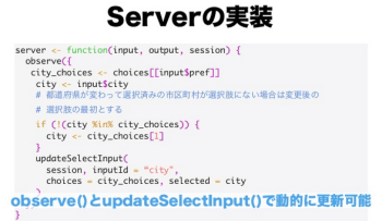
The main package that facilitates this in both R and Shiny is the
The There's not a whole lot you need to do to grab the results from another Another important component of the asynchronous framework in R is the
In a Shiny context, you can't use reactives inside a
You also need to carefully think about WHERE (as in which process)
Although the above code works in both cases, for some functions such as
Np_Ur: A Simple Shiny App in 30 Minutes!
I recommend going through his slides (also hosted on Shiny) as well as kashitan: Making {shiny} Maps with {leaflet}!
The first function:
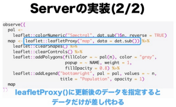
You can check out the documentation The second function:
The third function:
The last function:
okiyuki: Software Engineering for Shiny!
An extra section talked about various helpful packages for Shiny app
LTsigjit: Edit Your Photos with {shinyroom}!You might remember from a few months back,
In terms of actually building the Shiny app he used the {imager} package During the course of building the app,
flaty13: Reproducible Shiny with {shinymeta}!
The next step that is currently in development is to output an
Other talks
Food, Drinks, and Conclusion
Talks in English are also welcome so if you're ever in Tokyo come join To leave a comment for the author, please follow the link and comment on their blog: R by R(yo). R-bloggers.com offers daily e-mail updates about R news and tutorials about learning R and many other topics. Click here if you're looking to post or find an R/data-science job. Want to share your content on R-bloggers? click here if you have a blog, or here if you don't. This posting includes an audio/video/photo media file: Download Now | |||||||||||||||||||||||||||||||||||||||||||||||||||||||||||||||
| The Mysterious Case of the Ghost Interaction Posted: 29 Oct 2019 05:00 PM PDT [This article was first published on R on I Should Be Writing: Est. 1641, and kindly contributed to R-bloggers]. (You can report issue about the content on this page here) Want to share your content on R-bloggers? click here if you have a blog, or here if you don't. This spooky post was written in collaboration with Yoav Kessler (@yoav_kessler) and Naama Yavor (@namivor).. Experimental psychology is moving away from repeated-measures-ANOVAs, and towards linear mixed models (LMM1). LMMs have many advantages over rmANOVA, including (but not limited to):
This post will focus on this last point. Specifically, why you should always include main-effects when modeling interactions, and what happens if you don't (spooky). Fitting the Right (yet oh so wrong) ModelSay you've finally won that grant you submitted to study candy consumption during ghostly themed holidays. As part of your first study, you decide to measure the effects of costume type (scary / cute) and level of neighborhood decor (high / low levels of house decorations) on the total weight of collected candy (in Kg). A simple, yet informative 2-by-2 design. Being the serious scientist you are, you have several hypotheses:
It would only make sense to specify your statistical model accordingly – after all, why shouldn't your model represent your hypotheses? In R, such a model is described as And so, you fit the model:
As predicted, you find both a significant main effect for decor and the interaction decor \(\times\) costume, with the interaction explaining 40% of the variance in collected candy weight. So far so good – your results reflect your hypotheses! But then you plot your data, and to your horror you find…
It looks like there is no interaction at all! Your interaction was nothing more than a ghost! An apparition! How is this possible?? Where has all of variance explained by it gone???  What IS This?? In fact, had you fit the full model, you would have found:
The interaction actually explains 0% of the variance! And the effect of costume is the one that explains 40% of the variance!3 How could this be?? Have we angered Fisher's spirit somehow? What happened was that because we did not account for costume in our model, the variance explained by costume was swallowed by the interaction decor \(\times\) costume! The MathIf you find math too scary, feel free to skip to conclusion. Travel back to Intro to Stats, and recall that the interaction's sum-of-squares – \(SS_{A\times B}\) – is calculated as: \(SS_{A\times B} = (\bar{x}_{ij} – \bar{x}_{i.} – \bar{x}_{.j} + \bar{\bar{x}}_{..})^2\) This is a simplification of the following equation: \(SS_{A\times B} = \sum \sum (\bar{x}_{ij} – (\bar{x}_{i.} – \bar{\bar{x}}_{..}) – (\bar{x}_{.j} – \bar{\bar{x}}_{..}) + \bar{\bar{x}}_{..})^2\) Where \((\bar{x}_{i.} – \bar{\bar{x}}_{..})\) represents the main effect for \(A\) and \((\bar{x}_{.j} – \bar{\bar{x}}_{..})\) represents the main effect for \(B\). We can see that \(SS_{A\times B}\) represents the deviation from the additive model – i.e., it is the degree by which the observed cells' means deviate from what would be expected if there were only the two main effects. When we exclude the main effect of \(B\) from out model, we are telling our model that there is no need to estimate the main effect. That is, we set \((\bar{x}_{.j} – \bar{\bar{x}}_{..})=0\). The resulting \(SS_{A\times B}\) is computed not as above, but as: \(SS_{A\times B} = \sum \sum (\bar{x}_{ij} – (\bar{x}_{i.} – \bar{\bar{x}}_{..}) + \bar{\bar{x}}_{..})^2\) This formula represents the degree by which the observed cells' means deviate from what would be expected if there was only the main effect of \(A\). But now if the cells' means deviate in a way that would otherwise have been part of a main effect for \(B\), the cells' deviations from the main effect for \(A\) will now include the deviations that would otherwise have been accounted for by a main effect of \(B\)! This results in the main effect for \(B\) essentially getting "pooled" into \(SS_{A\times B}\). Furthermore, had you also excluded a main effect for \(A\), this effect too would have been "pooled" into the so-called \(A\times B\) interaction. In other words:
ConclusionSure, you can specify a model with no main effect and only interactions, but in such a case the interactions no longer mean what we expect them to mean. If we want interactions to represent deviation from the additive model, our model must also include the additive model! For simplicity's sake, this example has focused on a simple 2-by-2 between subject design, but the conclusions drawn here are relevant for any design in which a factor interacts with or moderates the effect of another factor or continuous variable.
To leave a comment for the author, please follow the link and comment on their blog: R on I Should Be Writing: Est. 1641. R-bloggers.com offers daily e-mail updates about R news and tutorials about learning R and many other topics. Click here if you're looking to post or find an R/data-science job. Want to share your content on R-bloggers? click here if you have a blog, or here if you don't. This posting includes an audio/video/photo media file: Download Now | |||||||||||||||||||||||||||||||||||||||||||||||||||||||||||||||
| Posted: 29 Oct 2019 12:00 PM PDT [This article was first published on R – Statistical Modeling, Causal Inference, and Social Science, and kindly contributed to R-bloggers]. (You can report issue about the content on this page here) Want to share your content on R-bloggers? click here if you have a blog, or here if you don't. Throw this onto the big pile of stats problems that are a lot more subtle than they seem at first glance. This all started when Lauren pointed me at the post Another way to see why mixed models in survey data are hard on Thomas Lumley's blog. Part of the problem is all the jargon in survey sampling—I couldn't understand Lumley's language of estimators and least squares; part of it is that missing data is hard. The full data model Imagine we have a a very simple population of To complete the Bayesian model, we'll assume a standard normal prior on Now we're not going to observe all Missing data Now let's assume the sample of
Now when we collect our sample, we'll do something like poll This situation arises in surveys, where non-response can bias results without careful adjustment (e.g., see Andrew's post on pre-election polling, Don't believe the bounce). So how do we do the careful adjustment? Approach 1: Weighted likelihood A traditional approach is to inverse weight the log likelihood terms by the inclusion probability, Thus if an item has a 20% chance of being included, its weight is 5. In Stan, we can code the weighted likelihood as follows (assuming pi is given as data). for (n in 1:N_obs) target += inv(pi[n]) * normal_lpdf(y[n] | mu, 2); If we optimize with the weighted likelihood, the estimates are unbiased (i.e., the expectation of the estimate Although the parameter estimates are unbiased, the same cannot be said of the uncertainties. The posterior intervals are too narrow. Specifically, this approach fails simulation-based calibration; for background on SBC, see Dan's blog post You better check yo self before you wreck yo self. One reason the intervals are too narrow is that we are weighting the data as if we had observed So my next thought was to standardize. Let's take the inverse weights and normalize so the sum of inverse weights is equal to Sure, we could keep fiddling weights in an ad hoc way for this problem until they were better calibrated empirically, but this is clearly the wrong approach. We're Bayesians and should be thinking generatively. Maybe that's why Lauren and Andrew kept telling me I should be thinking generatively (even though they work on a survey weighting project!). Approach 2: Missing data What is going on generativey? We poll Given that we know how Specifically, the This works. Here's the Stan program. data { int N_miss; int N_obs; vector[N_obs] y_obs; } parameters { real mu; vector[N_miss] y_miss; } model { // prior mu ~ normal(0, 1); // observed data likelihood y_obs ~ normal(mu, 2); 1 ~ bernoulli_logit(y_obs); // missing data likelihood and missingness y_miss ~ normal(mu, 2); 0 ~ bernoulli_logit(y_miss); } The Bernoulli sampling statements are vectorized and repeated for each element of y_obs and y_miss. The suffix _logit indicates the argument is on the log odds scale, and could have been written: for (n in 1:N_miss) 0 ~ bernoulli(y_miss[n] | inv_logit(y_miss[n])) And here's the simulation code, including a cheap run at SBC: library(rstan) rstan_options(auto_write = TRUE) options(mc.cores = parallel::detectCores(), logical = FALSE) printf <- function(msg, ...) { cat(sprintf(msg, ...)); cat("\n") } inv_logit <- function(u) 1 / (1 + exp(-u)) printf("Compiling model.") model <- stan_model('missing.stan') for (m in 1:20) { # SIMULATE DATA mu <- rnorm(1, 0, 1); N_tot <- 1000 y <- rnorm(N_tot, mu, 2) z <- rbinom(N_tot, 1, inv_logit(y)) y_obs <- y[z == 1] N_obs <- length(y_obs) N_miss <- N_tot - N_obs # COMPILE AND FIT STAN MODEL fit <- sampling(model, data = list(N_miss = N_miss, N_obs = N_obs, y_obs = y_obs), chains = 1, iter = 5000, refresh = 0) mu_ss <- extract(fit)$mu mu_hat <- mean(mu_ss) q25 <- quantile(mu_ss, 0.25) q75 <- quantile(mu_ss, 0.75) printf("mu = %5.2f in 50pct(%5.2f, %5.2f) = %3s; mu_hat = %5.2f", mu, q25, q75, ifelse(q25 <= mu && mu <= q75, "yes", "no"), mean(mu_ss)) } Here's some output with random seeds, with mu, mu_hat and 50% intervals and indicator of whether mu is in the 50% posterior interval. mu = 0.60 in 50pct( 0.50, 0.60) = no; mu_hat = 0.55 mu = -0.73 in 50pct(-0.67, -0.56) = no; mu_hat = -0.62 mu = 1.13 in 50pct( 1.00, 1.10) = no; mu_hat = 1.05 mu = 1.71 in 50pct( 1.67, 1.76) = yes; mu_hat = 1.71 mu = 0.03 in 50pct(-0.02, 0.08) = yes; mu_hat = 0.03 mu = 0.80 in 50pct( 0.76, 0.86) = yes; mu_hat = 0.81 The only problem I'm having is that this crashes RStan 2.19.2 on my Mac fairly regularly. Exercise How would the generative model differ if we polled members of the population at random until we got 1000 respondents? Conceptually it's more difficult in that we don't know how many non-resondents were approached on the way to 1000 respondents. This would be tricky in Stan as we don't have discrete parameter sampling---it'd have to be marginalized out. Lauren started this conversation saying it would be hard. It took me several emails, part of a Stan meeting, buttonholing Andrew to give me an interesting example to test, lots of coaching from Lauren, then a day of working out the above simulations to convince myself the weighting wouldn't work and code up a simple version that would work. Like I said, not easy. But at least doable with patient colleagues who know what they're doing. To leave a comment for the author, please follow the link and comment on their blog: R – Statistical Modeling, Causal Inference, and Social Science. R-bloggers.com offers daily e-mail updates about R news and tutorials about learning R and many other topics. Click here if you're looking to post or find an R/data-science job. Want to share your content on R-bloggers? click here if you have a blog, or here if you don't. This posting includes an audio/video/photo media file: Download Now | |||||||||||||||||||||||||||||||||||||||||||||||||||||||||||||||
| Posted: 29 Oct 2019 06:59 AM PDT [This article was first published on Blog: John C. Nash, and kindly contributed to R-bloggers]. (You can report issue about the content on this page here) Want to share your content on R-bloggers? click here if you have a blog, or here if you don't. There has been a campaign by members of the Canadian library community to ask international publishers to reduce prices to libraries for eBooks. If my experience in the scientific publishing arena is any guide, the publishers will continue to charge the maximum they can get until the marketplace — that is us — forces them to change or get out of business. This does not mean that the campaign is without merit. I just feel it needs to be augmented by some explorations of alternatives that could lead to a different ecosystem for writers and readers, possibly without traditional publishers. Where am I coming from?
How does this help libraries? First, I'd be really happy if libraries where my novels are of local interest would make them freely available. There are clearly some minor costs to doing this, but we are talking of a few tens of dollars in labour to add a web-page and a link or two, and some cents of storage cost. I offered my first novel, which involves Ottawa, to the Ottawa Public Library, but was told I would have to pay an external (indeed US) company for the DRM to be applied. But I offered an unlimited number of downloads! Is it surprising that I went to archive.org and obooko.com? And the library has fewer offerings for its readers, but also I miss out on local readers being offered my work. Second, I believe there are other authors whose motivations are not primarily financial who may be willing to offer their works in a similar fashion. My own motivations are to record anecdotes and events not otherwise easily accessed, if at all. I put these in a fictional shell to provide readability and structure. Given that obooko.com seems to be doing reasonably well, though some of the offerings are less than stellar, there are clearly other authors willing to make their works available to readers. Third, there may be authors willing to offer their works for free for a limited time to allow initiatives by libraries to be tried out, even if they do want or need to be remunerated eventually. What about the longer term? DRM imposes considerable costs on both libraries and readers. Whether it protects authors can be debated. Its main damage is that it cedes control of works from authors and readers to foreign, often very greedy, companies, whose interests are not in creative works but in selling software systems. Worse, it only really protects the income of those companies. All DRM schemes are breakable, though they are always a nuisance. Some workers talk of "social DRM" or watermarking. I believe this could be a useful tool. The borrower/buyer is identified on the work. I have done this with my books in the past, using a scheme developed to put a name on each page of student examination papers so each student had a unique paper. This avoided the need for strict invigilation, since copied answers could be wrong. In an ebook, the idea could be enhanced with invisible encoding of the name (steganography). However, each additional feature is another cost, another obstacle to getting the work to the reader. And no scheme is unbreakable. Publishers now insist on "renewal" of the license for an eBook. The library may not get a "reference" copy. Personally, I believe one of the important roles of libraries is to serve as repositories of works. A single disk can store an awful number of eBooks, so the cost is small. As a possibility, reading the archival copies could be restricted to in-library access only, but users would have a chance to verify material for study and reference purposes. Audiobooks require more storage, and are less easy to use for reference purposes, but could be similarly archived, as the audiobook reader's voice may be of interest. For a sustainable writer-library-reader system, there does need to be a way to reward writers. The current scheme, with DRM, counts downloads. This is costly to libraries. How many times have you abandoned a book after a few pages? This might be overcome with some sort of sampling mechanism providing more material than currently offered as a "tease". If eBooks are available in unlimited quantities, authors could actually benefit more. There are often temporary fads or surges of interest, or else book club members all want to read a title. At the moment, I know some club members will decide not to bother with a given book, or will find ways to "share". Clearly, libraries will not want to have open-ended costs, but it is likely that works will be temporarily popular. As I understand things, traditional publishers allow a fixed number of borrowings, so there is in essence a per-borrowing charge. In effect this is infinite for a never-borrowed work. Those of us in the non-traditional community who still want some reward might be happy with a smaller per-borrowing reward, and may also be willing to accept a cap or a per-year maximum or some similar arrangement that still keeps costs lower for the library. My view I want my work read. Readers want choice and diversity. Libraries want to grow the community of written work. It is time to think out of the DRM box.
To leave a comment for the author, please follow the link and comment on their blog: Blog: John C. Nash. R-bloggers.com offers daily e-mail updates about R news and tutorials about learning R and many other topics. Click here if you're looking to post or find an R/data-science job. Want to share your content on R-bloggers? click here if you have a blog, or here if you don't. This posting includes an audio/video/photo media file: Download Now | |||||||||||||||||||||||||||||||||||||||||||||||||||||||||||||||
| Posted: 29 Oct 2019 01:26 AM PDT [This article was first published on English – SmarterPoland.pl, and kindly contributed to R-bloggers]. (You can report issue about the content on this page here) Want to share your content on R-bloggers? click here if you have a blog, or here if you don't. Few days ago a new version of DALEX was accepted by CRAN (v 0.4.9). Here you will find short overview what was added/changed. DALEX is an R package with methods for visual explanation and exploration of predictive models. Major changes in the last version Verbose model wrapping Function explain() is now more verbose. During the model wrapping it checks the consistency of arguments. This works as unit tests for a model. This way most common problems with model exploration can be identified early during the exploration.
Support for new families of models We have added more convenient support for gbm models. The ntrees argument for predict_function is guessed from the model structure. Integration with other packages DALEX has now better integration with the auditor package. DALEX explainers can be used with any function form the auditor package. So, now you can easily create an ROC plot, LIFT chart or perform analysis of residuals. This way we have access to a large number of loss functions. Richer explainers Explainers have now new elements. Explainers store information about packages that were used for model development along with their versions. A bit of philosophy Cross-comparisons of models is tricky because predictive models may have very different structures and interfaces. DALEX is based on an idea of an universal adapter that can transform any model into a wrapper with unified interface that can be digest by any model agnostic tools. In this medium article you will find a longer overview of this philosophy. To leave a comment for the author, please follow the link and comment on their blog: English – SmarterPoland.pl. R-bloggers.com offers daily e-mail updates about R news and tutorials about learning R and many other topics. Click here if you're looking to post or find an R/data-science job. Want to share your content on R-bloggers? click here if you have a blog, or here if you don't. This posting includes an audio/video/photo media file: Download Now | |||||||||||||||||||||||||||||||||||||||||||||||||||||||||||||||
| Extracting basic Plots from Novels: Dracula is a Man in a Hole Posted: 29 Oct 2019 01:00 AM PDT [This article was first published on R-Bloggers – Learning Machines, and kindly contributed to R-bloggers]. (You can report issue about the content on this page here) Want to share your content on R-bloggers? click here if you have a blog, or here if you don't.
When you think about it the shape "Man in a Hole" (characters plunge into trouble and crawl out again) really is one of the most popular – even the Bible follows this simple script (see below)!
A colleague of mine, Professor Matthew Jockers from the University of Nebraska, has analyzed 50,000 novels and found out that Vonnegut was really up to something: there are indeed only half a dozen possible plots most novels follow. You can read more about this project here: The basic plots of fiction Professor Jockers has written a whole book about this topic: "The Bestseller Code". But what is even more mind-blowing than this unifying pattern of all stories is that you can do these analyses yourself – with any text of your choice! Professor Jockers made the A while ago I finished Dracula, the (grand-)father of all vampire and zombie stories. What a great novel that is! Admittedly it is a little slow-moving but the atmosphere is better than in any of the now popular TV series. Of course, I wanted to do an analysis of the publicly available Dracula text. The following code should be mostly self-explanatory. First the original text (downloaded from Project Gutenberg: Bram Stoker: Dracula) is broken down into separate sentences. After that the sentiment for each sentence is being evaluated and all the values smoothed out (by using some kind of specialized low pass filter). Finally the transformed values are plotted: library(syuzhet) dracula <- get_text_as_string("data/pg345.txt") Dracula <- get_sentences(dracula) Dracula_sent <- get_sentiment(Dracula, method = "bing") ft_values <- get_dct_transform(Dracula_sent, low_pass_size = 3, scale_range = TRUE) plot(ft_values, type = "l", main = "Dracula using Transformed Values", xlab = "Narrative Time", ylab = "Emotional Valence", col = "red") abline(h = 0)
In a way R has "read" the novel in no time and extracted the basic plot – pretty impressive, isn't it! As you can see the story follows the "Man in a Hole"-script rather exemplary, which makes sense because at the beginning everything seems to be fine and well, then Dracula appears and, of course, bites several protagonists, but in the end they catch and kill him – everything is fine again. THE END
…as a bonus, here is the plot that shows that the Bible also follows a simple "Man in a Hole" narrative (paradise, paradise lost, paradise regained). Fortunately, you can conveniently install the King James Bible as a package: https://github.com/JohnCoene/sacred # devtools::install_github("JohnCoene/sacred") library(sacred) KJV_sent <- get_sentiment(king_james_version$text, method = "bing") ft_values <- get_dct_transform(KJV_sent, low_pass_size = 3, scale_range = TRUE) plot(ft_values, type = "l", main = "King James Bible using Transformed Values", xlab = "Narrative Time", ylab = "Emotional Valence", col = "red") abline(h = 0)
Simple stories often work best! To leave a comment for the author, please follow the link and comment on their blog: R-Bloggers – Learning Machines. R-bloggers.com offers daily e-mail updates about R news and tutorials about learning R and many other topics. Click here if you're looking to post or find an R/data-science job. Want to share your content on R-bloggers? click here if you have a blog, or here if you don't. This posting includes an audio/video/photo media file: Download Now | |||||||||||||||||||||||||||||||||||||||||||||||||||||||||||||||
| (Re)introducing skimr v2 – A year in the life of an open source R project Posted: 28 Oct 2019 05:00 PM PDT [This article was first published on rOpenSci - open tools for open science, and kindly contributed to R-bloggers]. (You can report issue about the content on this page here) Want to share your content on R-bloggers? click here if you have a blog, or here if you don't. We announced the testing version of skimr v2 on Wait, what is a "skimr"?skimr is an R package for summarizing your data. It extends tidyverse packages, skimr is also on Setting the stageBefore we can talk about the last year of skimr development, we need to lay out skimr was originally an About six months later, we released our first version on CRAN. The time between Getting the package on CRAN opened the gates for bug reports and feature A month after finishing the peer review (and six months after the process Just kidding! We love our little histograms, even when they don't love us back! Getting it rightUnder normal circumstances (i.e. not during a hackathon), most software
Better internal data structuresIn v1, skimr stored all of its data in a "long format", data frame. Although Big ups to anyone who looked at the rendered output and saw that this was how Now, working with skimr is a bit more sane. And It's still not perfect, as you need to rely on a pseudo-namespace to refer to There's a couple of other nuances here:
Manipulating internal dataA better representation of internal data comes with better tools for reshaping You can undo a call to Last, with support something close to the older format with the Working with dplyrUsing skimr in a In practice, this means that you can coerce it into a different type through To get around this, we've added some helper functions and methods. The more Configuring and extending skimrMost of skimr's magic, to One big one is customization. We like the skimr defaults, but that doesn't Those of you familiar with customizing
Yes! A function factory.
The other big change is how we now handle different data types. Although many While it was required in Even if you don't go the full route of supporting a new data type, creating a Using skimr in other contextsIn skimr v1, we developed some slightly hacky approaches to getting nicer
Variable type: factor
Variable type: numeric
You get a nice html version of both the summary header and the skimr subtables In this context, you configure the output the same way you handle other This means that we're dropping direct support for We also have a similarly-nice rendered output in Wait, that took over a year?Well, we think that's a lot! But to be fair, it wasn't exactly simple to keep up Even so, these are just the highlights in the normal ebb and flow of this sort We're really excited about this next step in the skimr journey. We've put a huge If you want to learn more about skimr, check out our To leave a comment for the author, please follow the link and comment on their blog: rOpenSci - open tools for open science. R-bloggers.com offers daily e-mail updates about R news and tutorials about learning R and many other topics. Click here if you're looking to post or find an R/data-science job. Want to share your content on R-bloggers? click here if you have a blog, or here if you don't. This posting includes an audio/video/photo media file: Download Now | |||||||||||||||||||||||||||||||||||||||||||||||||||||||||||||||
| Posted: 28 Oct 2019 05:00 PM PDT [This article was first published on Dyfan Jones Brain Dump HQ, and kindly contributed to R-bloggers]. (You can report issue about the content on this page here) Want to share your content on R-bloggers? click here if you have a blog, or here if you don't. RBloggers|RBloggers-feedburner Intro:For a long time I have found it difficult to appreciate the benefits of "cloud compute" in my R model builds. This was due to my initial lack of understanding and the setting up of R on cloud compute environments. When I noticed that AWS was bringing out a new product AWS Sagemaker, the possiblities of what it could provide seemed like a dream come true.
A question about AWS Sagemake came to mind: Does it work for R developers??? Well…not exactly. True it provides a simple way to set up an R environment in the cloud but it doesn't give the means to access other AWS products for example AWS S3 and AWS Athena out of the box. However for Python this is not a problem. Amazon has provided a Software Development Kit (SDK) for Python called It isn't all bad news, RStudio has developed a package called AWS interfaces for R:
| |||||||||||||||||||||||||||||||||||||||||||||||||||||||||||||||
| Sept 2019: “Top 40” New R Packages Posted: 28 Oct 2019 05:00 PM PDT [This article was first published on R Views, and kindly contributed to R-bloggers]. (You can report issue about the content on this page here) Want to share your content on R-bloggers? click here if you have a blog, or here if you don't. One hundred and thirteen new packages made it to CRAN in September. Here are my "Top 40" picks in eight categories: Computational Methods, Data, Economics, Machine Learning, Statistics, Time Series, Utilities, and Visualization. Computational MethodseRTG3D v0.6.2: Provides functions to create realistic random trajectories in a 3-D space between two given fixed points (conditional empirical random walks), based on empirical distribution functions extracted from observed trajectories (training data), and thus reflect the geometrical movement characteristics of the mover. There are several small vignettes, including sample data sets, linkage to the
freealg v1.0: Implements the free algebra in R: multivariate polynomials with non-commuting indeterminates. See the vignette for the math. HypergeoMat v3.0.0: Implements Koev & Edelman's algorithm (2006) to evaluate the hypergeometric functions of a matrix argument, which appear in random matrix theory. There is a vignette. opart v2019.1.0: Provides a reference implementation of standard optimal partitioning algorithm in C using square-error loss and Poisson loss functions as described by Maidstone (2016), Hocking (2016), Rigaill (2016), and Fearnhead (2016) that scales quadratically with the number of data points in terms of time-complexity. There are vignettes for Gaussian and Poisson squared error loss.
Datacde v0.4.1: Facilitates searching, download and plotting of Water Framework Directive (WFD) reporting data for all water bodies within the UK Environment Agency area. This package has been peer-reviewed by rOpenSci. There is a Getting Started Guide and a vignette on output reference.
eph v0.1.1: Provides tools to download and manipulate data from the Argentina Permanent Household Survey. The implemented methods are based on INDEC (2016). leri v0.0.1: Fetches Landscape Evaporative Response Index (LERI) data using the
rwhatsapp v0.2.0: Provides functions to parse and digest history files from the popular messenger service WhatsApp. There is a vignette.
tidyUSDA v0.2.1: Provides a consistent API to pull United States Department of Agriculture census and survey data from the National Agricultural Statistics Service (NASS) QuickStats service. See the vignette. Economicsbunching v0.8.4: Implements the bunching estimator from economic theory for kinks and knots. There is a vignette on Theory, and another with Examples.
fixest v0.1.2: Provides fast estimation of econometric models with multiple fixed-effects, including ordinary least squares (OLS), generalized linear models (GLM), and the negative binomial. The method to obtain the fixed-effects coefficients is based on Berge (2018). There is a vignette. raceland v1.0.3: Implements a computational framework for a pattern-based, zoneless analysis, and visualization of (ethno)racial topography for analyzing residential segregation and racial diversity. There is a vignette describing the Computational Framework, one describing Patterns of Racial Landscapes, and a third on SocScape Grids.
Machine Learningbiclustermd v0.1.0: Implements biclustering, a statistical learning technique that simultaneously partitions, and clusters rows and columns of a data matrix in a manner that can deal with missing values. See the vignette for examples.
bbl v0.1.5: Implements supervised learning using Boltzmann Bayes model inference, enabling the classification of data into multiple response groups based on a large number of discrete predictors that can take factor values of heterogeneous levels. See Woo et al. (2016) for background, and the vignette for how to use the package.
corporaexplorer v0.6.3: Implements Shiny apps to dynamically explore collections of texts. Look here for more information. fairness v1.0.1: Offers various metrics to assess and visualize the algorithmic fairness of predictive and classification models using methods described by Calders and Verwer (2010), Chouldechova (2017), Feldman et al. (2015), Friedler et al. (2018), and Zafar et al. (2017). There is a tutorial for the package.
imagefluency v0.2.1: Provides functions to collect image statistics based on processing fluency theory that include scores for several basic aesthetic principles that facilitate fluent cognitive processing of images: contrast, complexity / simplicity, self-similarity, symmetry, and typicality. See Mayer & Landwehr (2018) and Mayer & Landwehr (2018) for the theoretical background, and the vignette for an introduction.
ineqJD v1.0: Provides functions to compute and decompose Gini, Bonferroni, and Zenga 2007 point and synthetic concentration indexes. See Zenga M. (2015), Zenga & Valli (2017), and Zenga & Valli (2018) for more information. lmds v0.1.0: Implements Landmark Multi-Dimensional Scaling (LMDS), a dimensionality reduction method scaleable to large numbers of samples, because rather than calculating a complete distance matrix between all pairs of samples, it only calculates the distances between a set of landmarks and the samples. See the README for an example. modelStudio v0.1.7: Implements an interactive platform to help interpret machine learning models. There is a vignette, and look here for a demo of the interactive features.
nlpred v1.0: Provides methods for obtaining improved estimates of non-linear cross-validated risks obtained using targeted minimum loss-based estimation, estimating equations, and one-step estimation. Cross-validated area under the receiver operating characteristics curve ( LeDell sr al. (2015) ) and other metrics are included. There is a vignette on small sample estimates. pyMTurkR v1.1: Provides access to the latest Amazon Mechanical Turk' ('MTurk') Requester API (version '2017–01–17'), replacing the now deprecated stagedtrees v1.0.0: Creates and fits staged event tree probability models, probabilistic graphical models capable of representing asymmetric conditional independence statements among categorical variables. See Görgen et al. (2018), Thwaites & Smith (2017), Barclay et al. (2013), and Smith & Anderson](doi:10.1016/j.artint.2007.05.004) for background, and look here for and overview.
Statisticsconfoundr v1.2: Implements three covariate-balance diagnostics for time-varying confounding and selection-bias in complex longitudinal data, as described in Jackson (2016) and Jackson (2019). There is a Demo vignette and another Describing Selection Bias from Dependent Censoring
distributions3 v0.1.1: Provides tools to create and manipulate probability distributions using S3. Generics
dobin v0.8.4: Implements a dimension reduction technique for outlier detection, which constructs a set of basis vectors for outlier detection that bring outliers to the forefront using fewer basis vectors. See Kandanaarachchi & Hyndman (2019) for background, and the vignette for a brief introduction.
glmpca v0.1.0: Implements a generalized version of principal components analysis (GLM-PCA) for dimension reduction of non-normally distributed data, such as counts or binary matrices. See Townes et al. (2019) and Townes (2019) for details, and the vignette for examples. immuneSIM v0.8.7: Provides functions to simulate full B-cell and T-cell receptor repertoires using an in-silico recombination process that includes a wide variety of tunable parameters to introduce noise and biases. See Weber et al. (2019) for background, and look here for information about the package.
irrCAC v1.0: Provides functions to calculate various chance-corrected agreement coefficients (CAC) among two or more raters, including Cohen's kappa, Conger's kappa, Fleiss' kappa, Brennan-Prediger coefficient, Gwet's AC1/AC2 coefficients, and Krippendorff's alpha. There are vignettes on benchmarking, Calculating Chance-corrected Agreement Coefficients, and Computing weighted agreement coefficients. LPBlg v1.2: Provides functions that estimate a density and derive a deviance test to assess if the data distribution deviates significantly from the postulated model, given a postulated model and a set of data. See Algeri S. (2019) for details. SynthTools v1.0.0: Provides functions to support experimentation with partially synthetic data sets. Confidence interval and standard error formulas have options for either synthetic data sets or multiple imputed data sets. For more information, see Reiter & Raghunathan (2007). Time Seriesfable v0.1.0: Provides a collection of commonly used univariate and multivariate time series forecasting models, including automatically selected exponential smoothing (ETS) and autoregressive integrated moving average (ARIMA) models. There is an Introduction and a vignette on transformations.
nsarfima v0.1.0.0: Provides routines for fitting and simulating data under autoregressive fractionally integrated moving average (ARFIMA) models, without the constraint of stationarity. Two fitting methods are implemented: a pseudo-maximum likelihood method and a minimum distance estimator. See Mayoral (2007) and Beran (1995) for reference. Utilitiesnc v2019.9.16: Provides functions for extracting a data table (row for each match, column for each group) from non-tabular text data using regular expressions. Patterns are defined using a readable syntax that makes it easy to build complex patterns in terms of simpler, re-usable sub-patterns. There is a vignette on capture first match and another on capture all match. pins v0.2.0: Provides functions that "pin" remote resources into a local cache in order to work offline, improve speed, avoid recomputing, and discover and share resources in local folders, queryparser v0.1.1: Provides functions to translate SQL rawr v0.1.0: Retrieves pure R code from popular R websites, including github, kaggle, datacamp, and R blogs made using blogdown. VisualizationFunnelPlotR v0.2.1: Implements Spiegelhalter (2005) Funnel plots for reporting standardized ratios, with overdispersion adjustment. The vignette offers examples.
ggBubbles v0.1.4: Implements mini bubble plots to display more information for discrete data than traditional bubble plots do. The vignette provides examples.
gghalves v0.0.1: Implements a
To leave a comment for the author, please follow the link and comment on their blog: R Views. R-bloggers.com offers daily e-mail updates about R news and tutorials about learning R and many other topics. Click here if you're looking to post or find an R/data-science job. Want to share your content on R-bloggers? click here if you have a blog, or here if you don't. This posting includes an audio/video/photo media file: Download Now | |||||||||||||||||||||||||||||||||||||||||||||||||||||||||||||||
| Posted: 28 Oct 2019 05:00 PM PDT [This article was first published on Posts on R-hub blog, and kindly contributed to R-bloggers]. (You can report issue about the content on this page here) Want to share your content on R-bloggers? click here if you have a blog, or here if you don't. When writing unit tests for a package, you might find yourself wondering about how to best test the behaviour of your package
or you might even wonder how to test at least part of that package of yours that calls a web API or local database… without accessing the web API or local database during testing. In some of these cases, the programming concept you're after is mocking, i.e. making a function act as if something were a certain way! In this blog post we shall offer a round-up of resources around mocking, or not mocking, when unit testing an R package.
Please keep reading, do not flee to Twitter! Packages for mockingGeneral mockingNowadays, when using Let's also look at a real life example, from What happens after the call to Instead of directly defining the return value as is the case in this example, one could stub the function with a function, as seen in one of the tests for the To find more examples of how to use Web mockingIn the case of a package doing HTTP requests, you might want to test what happens when an error code is received for instance. To do that, you can use either Temporarily modify the global stateTo test what happens when, say, an environment variable has a particular value, one can set it temporarily within a test using the To mock or… not to mockSometimes, you might not need mocking and can resort to an alternative approach instead, using the real thing/situation. You could say it's a less "unit" approach and requires more work. Fake input dataFor say a plotting or modelling library, you can tailor-make data. Comparing approaches or packages for creating fake data are beyond the scope of this post, so let's just name a few packages: Stored data from a web API / a databaseAs explained in this discussion about testing web API packages, when testing a package accessing and munging web data you might want to separate testing of the data access and of the data munging, on the one hand because failures will be easier to trace back to a problem in the web API vs. your code, on the other hand to be able to selectively turn off some tests based on internet connection, the presence of an API key, etc. Storing and replaying HTTP requests is supported by: What about applying the same idea to packages using a database connection?
Different operating systemsSay you want to be sure your packages builds correctly on another operating system… you can use R-hub package builder Different system configurations or librariesRegarding the case where you want to test your package when a suggested dependency is or is not installed, you can use the configuration script of a continuous integration service to have at least one build without that dependency:
ConclusionIn this post we offered a round-up of resources around mocking when unit testing R packages, as well as around not mocking. To learn about more packages for testing your package, refer to the list published on Locke Data's blog. Now, what if you're not sure about the best approach for that quirky thing you want to test, mocking or not mocking, and how exactly? Well, you can fall back on two methods: Reading the source code of other packages, and Asking for help! Good luck! To leave a comment for the author, please follow the link and comment on their blog: Posts on R-hub blog. R-bloggers.com offers daily e-mail updates about R news and tutorials about learning R and many other topics. Click here if you're looking to post or find an R/data-science job. Want to share your content on R-bloggers? click here if you have a blog, or here if you don't. This posting includes an audio/video/photo media file: Download Now | |||||||||||||||||||||||||||||||||||||||||||||||||||||||||||||||
| Any one interested in a function to quickly generate data with many predictors? Posted: 28 Oct 2019 05:00 PM PDT [This article was first published on ouR data generation, and kindly contributed to R-bloggers]. (You can report issue about the content on this page here) Want to share your content on R-bloggers? click here if you have a blog, or here if you don't. A couple of months ago, I was contacted about the possibility of creating a simple function in I'm presenting a new function here as a work-in-progress. I am putting it out there in case other folks have opinions about what might be most useful; feel free to let me know if you do. If not, I am likely to include something very similar to this in the next iteration of Function genMultPredIn its latest iteration, the new function has three interesting arguments. The first two are The third interesting argument is Currently, the outcome can only have one of three distributions: normal, binomial, or Poisson. One possible enhancement would be to allow the distributions of the predictors to have more flexibility. However, I'm not sure the added complexity would be worth it. Again, you could always take the more standard Here's the function, in case you want to take a look under the hood: A brief exampleHere is an example with 7 normally distributed covariates and 4 binary covariates. Only 3 of the continuous covariates and 2 of the binary covariates will actually be predictive. The function returns a list of two objects. The first is a data.table containing the generated predictors and outcome: The second object is the set of coefficients that determine the average response conditional on the predictors: Finally, we can "recover" the original coefficients with linear regression: Here's a plot showing the 95% confidence intervals of the estimates along with the true values. The yellow lines are covariates where there is truly no association.
Addendum: correlation among predictorsHere is a pair of examples using the To leave a comment for the author, please follow the link and comment on their blog: ouR data generation. R-bloggers.com offers daily e-mail updates about R news and tutorials about learning R and many other topics. Click here if you're looking to post or find an R/data-science job. Want to share your content on R-bloggers? click here if you have a blog, or here if you don't. This posting includes an audio/video/photo media file: Download Now | |||||||||||||||||||||||||||||||||||||||||||||||||||||||||||||||
| Posted: 28 Oct 2019 10:18 AM PDT [This article was first published on R on kieranhealy.org, and kindly contributed to R-bloggers]. (You can report issue about the content on this page here) Want to share your content on R-bloggers? click here if you have a blog, or here if you don't. The other week I took a few publicly-available datasets that I use for teaching data visualization and bundled them up into an R package called Using this data, I made a poster called Dogs of New York. It's a small multiple map of the relative prevalence of the twenty five most common dog breeds in the city, based on information from the city's dog license database. This morning, reflecting on a series of conversations I had with people about the original poster, I tweaked it a little further. In the original version, I used a discrete version of one of the Viridis palettes, initially the "Inferno" variant, and subsequently the "Plasma" one. These palettes are really terrific in everyday use for visualizations of all kinds, because they are vivid, colorblind-friendly, and perceptually uniform across their scale. I use them all the time, for instance with the Mortality in France poster I made last year. When it came to using this palette in a map, though, I ran into an interesting problem. Here's a detail from the "Plasma" palette version of the poster.  Detail from the Plasma version of Dogs of New York Now, these colors are vivid. But when I showed it to people, opinion was pretty evenly split between people who intuitively saw the darker, purplish areas as signifying "more", and people who intuitively saw the warmer, yellowish areas as signifying "more". So, for example, a number of people asked if I could make the map with the colors range flipped, with yellow meaning "more" or "high" (and indeed, in the very first version of the map I originally had done this). A friend with conflicting intuitions incisively noted that she associated darker colors with "more", in contrast to lighter colors, but also associated warmer colors with "more". The fact that the scale moved from a cooler, darker color through to a different, warmer, lighter color was thus confusing. The warm and vivid quality of the yellow end of the Plasma spectrum seemed to be particularly prone to this confusion. I think the small-multiple character of the graph exacerbated this confusion. It shows the selected dog breeds from most (top left) to least (bottom right) common, whereas the guide to the scale (in the top right) showed the scale running from low to high values, or least to most common. In the end, after a bit of experimentation I decided to redo the figure in a one-hue HCL scale, the "Oranges" palette from the Colorspace package. I also reversed the guide and added a few other small details to aid the viewer in interpreting the graph. Here's the final version.  Dogs of New York The palette isn't quite as immediately vivid as the Viridis version, but it seems to solve the problems of interpretation, and that's more important. The image is made to be blown up to quite a large size, which I plan on doing myself. To that end, here's a PDF version of the poster as well. To leave a comment for the author, please follow the link and comment on their blog: R on kieranhealy.org. R-bloggers.com offers daily e-mail updates about R news and tutorials about learning R and many other topics. Click here if you're looking to post or find an R/data-science job. Want to share your content on R-bloggers? click here if you have a blog, or here if you don't. This posting includes an audio/video/photo media file: Download Now | |||||||||||||||||||||||||||||||||||||||||||||||||||||||||||||||
| Spelunking macOS ‘ScreenTime’ App Usage with R Posted: 28 Oct 2019 07:33 AM PDT [This article was first published on R – rud.is, and kindly contributed to R-bloggers]. (You can report issue about the content on this page here) Want to share your content on R-bloggers? click here if you have a blog, or here if you don't. Apple has brought Screen Time to macOS for some time now and that means it has to store this data somewhere. Thankfully, Sarah Edwards has foraged through the macOS filesystem for us and explained where these bits of knowledge are in her post, Knowledge is Power! Using the macOS/iOS knowledgeC.db Database to Determine Precise User and Application Usage, which ultimately reveals the data lurks in Today, we'll show how to work with this database in R and the {tidyverse} to paint our own pictures of application usage. There are quite a number of tables in the That visual schema was created in OmniGraffle via a small R script that uses the OmniGraffle automation framework. The OmniGraffle source files are also available upon request. Most of the interesting bits (for any tracking-related spelunking) are in the There are a few ways to do this in {tidyverse} R. The first is an extended straight SQL riff off of one of Sarah's original queries: Before explaining what that query does, let's rewrite it {dbplyr}-style: What we're doing is pulling out the day of week, start/end usage times & timezone info, app bundle id, source of the app interactions and the total usage time for each entry along with when that entry was created. We need to do some maths since Apple stores time-y whime-y info in its own custom format, plus we need to convert numeric DOW to labeled DOW. The bundle ids are pretty readable, but they're not really intended for human consumption, so we'll make a translation table for the bundle id to app name by using the The usage info goes back ~30 days, so let's do a quick summary of the top 10 apps and their total usage (in hours): There's a YUGE flaw in the current way macOS tracks application usage. Unlike iOS where apps really don't run simultaneously (with iPadOS they kinda can/do, now), macOS apps are usually started and left open along with other apps. Apple doesn't do a great job identifying only active app usage activity so many of these usage numbers are heavily inflated. Hopefully that will be fixed by macOS 10.15. We have more data at our disposal, so let's see when these apps get used. To do that, we'll use segments to plot individual usage tracks and color them by weekday/weekend usage (still limiting to top 10 for blog brevity): I'm not entirely sure "on this Mac" is completely accurate since I think this syncs across all active Screen Time devices due to this (n is in seconds): The "Other" appears to be the work-dev Mac but it doesn't have the identifier mapped so I think that means it's the local one and that the above chart is looking at Screen Time across all devices. I literally (right before this sentence) enabled Screen Time on my iPhone so we'll see if that ends up in the database and I'll post a quick update if it does. We'll take one last look by day of week and use a heatmap to see the results: I really need to get into the habit of using the RStudio Server access features of RSwitch over Chrome so I can get RSwitch into the top 10, but some habits (and bookmarks) die hard. FINApple's Screen Time also tracks "category", which is something we can pick up from each application's embedded metadata. We'll do that in a follow-up post along with seeing whether we can capture iOS usage now that I've enabled Screen Time on those devices as well. Keep spelunking the To leave a comment for the author, please follow the link and comment on their blog: R – rud.is. R-bloggers.com offers daily e-mail updates about R news and tutorials about learning R and many other topics. Click here if you're looking to post or find an R/data-science job. Want to share your content on R-bloggers? click here if you have a blog, or here if you don't. This posting includes an audio/video/photo media file: Download Now | |||||||||||||||||||||||||||||||||||||||||||||||||||||||||||||||
| The Chaos Game: an experiment about fractals, recursivity and creative coding Posted: 28 Oct 2019 06:00 AM PDT [This article was first published on R – Fronkonstin, and kindly contributed to R-bloggers]. (You can report issue about the content on this page here) Want to share your content on R-bloggers? click here if you have a blog, or here if you don't.
You have a pentagon defined by its five vertex. Now, follow these steps:
If you repeat these steps 10 milion times, you will obtain this stunning image: I love the incredible ability of maths to create beauty. More concretely, I love the fact of how repeating extremely simple operations can bring you to unexpected places. Would you expect that the image created with the initial naive algorithm would be that? I wouldn't. Even knowing the result I cannot imagine how those simple steps can produce it. The image generated by all the points repeat itself at different scales. This characteristic, called self-similarity, is property of fractals and make them extremely attractive. Step 2 is the key one to define the shape of the image. Apart of comparing two previous vertex as it's defined in the algorithm above, I implemented two other versions:
These images are the result of applying the three versions of the algorithm to a square, a pentagon, a hexagon and a heptagon (a row for each polygon and a column for each algorithm): From a technical point of view I used Some days ago, I gave a tutorial at the coding club of the University Carlos III in Madrid where we worked with the integration of C++ and R to create beautiful images of strange attractors. The tutorial and the code we developed is here. You can also find the code of this experiment here. Enjoy! To leave a comment for the author, please follow the link and comment on their blog: R – Fronkonstin. R-bloggers.com offers daily e-mail updates about R news and tutorials about learning R and many other topics. Click here if you're looking to post or find an R/data-science job. Want to share your content on R-bloggers? click here if you have a blog, or here if you don't. This posting includes an audio/video/photo media file: Download Now |


.PNG?w=350)


 items with values normally distributed members with standard deviation known to be 2,
 \ \textrm{for} \ i \in 1:N^{\textrm{pop}}.")
 ,
,.")
 , but only a sample of the
  items from the population, and for each item
  , there is a probability
  that the item will be included in the sample. We'll take the log odds of inclusion to be equal to the item's value,
 ") .
. people from the population, but each person
  observations, with
  observations missing.
.")
 is the true value
  ). This is borne out in simulation.
 That also fails. The posterior intervals are still too narrow under simulation.
  , we can just model everything (in the real world, this stuff is really hard and everything's estimated jointly).
 representing how they would've responded had they responded. We also model response, so we have an extra term
 )") for the unobserved values and an extra term
for the unobserved values and an extra term )") for the observed values.
for the observed values.


 (The talented Sharla did end up using mocking for
 or maybe a


| You are subscribed to email updates from R-bloggers. To stop receiving these emails, you may unsubscribe now. | Email delivery powered by Google |
| Google, 1600 Amphitheatre Parkway, Mountain View, CA 94043, United States | |
Comments
Post a Comment